3.8.2

TinkerPop Sample Data

gremlin standing

TinkerPop bundles a small collection of sample graphs, often called "toy graphs", that appear throughout the reference documentation, the tutorials, and the test suites. They are deliberately small and self-contained so that a traversal can be read alongside the data it operates on, and they are available in every distribution without any external data source or configuration. Each graph is constructed by a factory method on TinkerFactory and also ships as data files under the data/ directory of the distribution in the GraphSON, GraphML, and Gryo formats.

This book serves as a reference for those graphs. Each section describes one graph: the nature of its data, where it came from, and the kinds of problems it illustrates best. Every graph is then given a schema expressed in GQL Graph Types, a declarative notation that states the node and edge labels a graph may contain, their properties and value types, and how edges connect the nodes. Finally, each section presents Gremlin examples that exercise the data and demonstrate the traversal patterns the graph was designed to teach.

The examples in this book are executable and run against the corresponding graph at build time, so their results are the actual output produced by the graph. The same graphs are available in the Gremlin Console through TinkerFactory, which makes it convenient to follow along and experiment with variations of the queries shown here.

The Modern Graph

The modern graph is the canonical example graph of Apache TinkerPop and the one used for the majority of the examples throughout the documentation. It models a small community of people and the software they created: marko, vadas, josh, and peter are people, while lop and ripple are software projects written in Java. People are connected to one another by knows edges and to software by created edges, and both kinds of edge carry a weight that indicates the strength of the relationship.

The graph originates in the "classic" toy graph that shipped with TinkerPop 2.x. It preserves that same six-vertex, six-edge structure but adopts the 3.x feature of vertex labels, distinguishing person vertices from software vertices rather than leaving every vertex unlabeled. Its small size and mix of two vertex labels and two edge labels make it well suited to demonstrating the fundamentals of Gremlin: navigating between adjacent vertices, filtering on labels and properties, and working with edge properties. It is created with TinkerFactory.createModern() and ships as data/tinkerpop-modern.*.

Figure 1. The Modern Graph

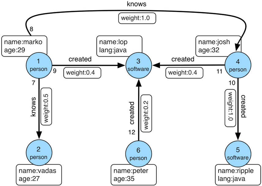
Schema

-- node types
(:person => { name :: STRING NOT NULL, age :: INT }),
(:software => { name :: STRING NOT NULL, lang :: STRING }),

-- edge types
(:person)-[:knows { weight :: DOUBLE }]->(:person),
(:person)-[:created { weight :: DOUBLE }]->(:software)

The weight property on both edge labels is a double-precision floating point value. This is one of the few differences from the older classic graph, where the same weight is a single-precision float.

Examples

The examples below introduce the people, then follow the two edge labels to explore who knows whom and who created what.

console groovy

gremlin> g.V().hasLabel('person').valueMap('name','age') // (1)
==>[name:[marko],age:[29]]
==>[name:[vadas],age:[27]]
==>[name:[josh],age:[32]]
==>[name:[peter],age:[35]]
gremlin> g.V().hasLabel('software').values('name') // (2)
==>lop
==>ripple
gremlin> g.V().has('person','name','marko').out('knows').values('name') // (3)
==>vadas
==>josh
gremlin> g.V().has('person','name','marko').out('created').values('name') // (4)
==>lop

g.V().hasLabel('person').valueMap('name','age') // (1)
g.V().hasLabel('software').values('name') // (2)
g.V().has('person','name','marko').out('knows').values('name') // (3)
g.V().has('person','name','marko').out('created').values('name') // (4)

This example runs against the modern graph.

The four people in the graph, each with a name and an age.
The two software projects. Software vertices carry a lang property rather than an age.
The people that marko knows, reached by following outgoing knows edges.
The software that marko created, reached by following outgoing created edges.

Because created edges point from people to software, the incoming direction of that same label identifies the authors of each project. Grouping by the software name summarizes who contributed to what.

console groovy

gremlin> g.V().hasLabel('software').
               group().
                 by('name').
                 by(__.in('created').values('name').fold()) // (1)
==>[ripple:[josh],lop:[marko,josh,peter]]

g.V().hasLabel('software').
      group().
        by('name').
        by(__.in('created').values('name').fold()) // (1)

This example runs against the modern graph.

For each software project, collect the names of the people who created it. Both lop and ripple are reached through created edges, and lop has more than one author.

The weight on a created edge records how much of a project a person contributed. Traversing the edge itself, rather than stepping straight to the adjacent vertex, makes that value available.

console groovy

gremlin> g.V().has('software','name','lop').
               inE('created').as('contribution'). // (1)
               outV().as('contributor').
               select('contributor','contribution').
                 by('name').
                 by('weight') // (2)
==>[contributor:marko,contribution:0.4]
==>[contributor:josh,contribution:0.4]
==>[contributor:peter,contribution:0.2]

g.V().has('software','name','lop').
      inE('created').as('contribution'). // (1)
      outV().as('contributor').
      select('contributor','contribution').
        by('name').
        by('weight') // (2)

This example runs against the modern graph.

Step onto the incoming created edges of lop and label them so the edge property can be selected later.
Pair each contributor’s name with the weight of their contribution to lop.

The Crew Graph

The crew graph models a group of contributors and the software they work on. marko, stephen, matthias, and daniel are people, while gremlin and tinkergraph are software. People develops and uses software, the develops edge records the year work began and the uses edge records a skill level, and one piece of software traverses another.

The graph was created to provide examples and test coverage for the structural features introduced in TinkerPop 3.x, and it is the reference example for three of them. First, a person’s location is a multi-property: each person has held several locations over time, so the single location key holds a list of values. Second, each location value carries meta-properties, startTime and an optional endTime, that record the span during which the person lived there. A location with no endTime is the person’s current one. Third, the graph itself carries graph variables that hold metadata about the graph. These features make the crew graph the right choice for demonstrating multi-properties, meta-properties, and graph variables. It is created with TinkerFactory.createTheCrew() and ships as data/tinkerpop-crew.*.

Figure 2. The Crew Graph

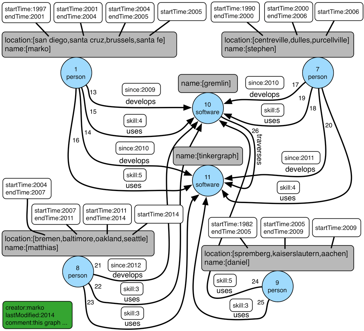
Schema

-- node types
(:person => { name :: STRING NOT NULL, location :: LIST<STRING> }),
(:software => { name :: STRING NOT NULL }),

-- edge types
(:person)-[:develops { since :: INT }]->(:software),
(:person)-[:uses { skill :: INT }]->(:software),
(:software)-[:traverses]->(:software)

GQL Graph Types describes the shape of vertices and edges but does not model every TinkerPop structural feature. The location multi-property is captured above as a LIST<STRING>, but the startTime and endTime meta-properties attached to each individual location value have no representation in the schema language, because meta-properties are properties on a property rather than on the vertex. The graph variables creator, lastModified, and comment are likewise metadata about the graph as a whole and fall outside the node and edge type definitions. Both are demonstrated in the examples below.

Examples

Because location is a multi-property whose values carry meta-properties, the current location of each person is the location value that has no endTime.

console groovy

gremlin> g.V().as('a').
               properties('location').as('b').
               hasNot('endTime').as('c'). // (1)
               select('a','b','c').by('name').by(value).by('startTime') // (2)
==>[a:marko,b:santa fe,c:2005]
==>[a:stephen,b:purcellville,c:2006]
==>[a:matthias,b:seattle,c:2014]
==>[a:daniel,b:aachen,c:2009]

g.V().as('a').
      properties('location').as('b').
      hasNot('endTime').as('c'). // (1)
      select('a','b','c').by('name').by(value).by('startTime') // (2)

This example runs against the crew graph.

Keep only the location value that has no endTime meta-property, which is the current one.
Report each person’s name, current location value, and the startTime meta-property that records when they moved there.

The full residence history of a person is obtained by ordering all of their location values by startTime. A location that is still current has no endTime, so coalesce() supplies a stand-in value in that case.

console groovy

gremlin> g.V().has('person','name','daniel').
               properties('location'). // (1)
               order().by('startTime',asc).
               project('city','from','to').
                 by(value).
                 by('startTime').
                 by(coalesce(values('endTime'), constant('present'))) // (2)
==>[city:spremberg,from:1982,to:2005]
==>[city:kaiserslautern,from:2005,to:2009]
==>[city:aachen,from:2009,to:present]

g.V().has('person','name','daniel').
      properties('location'). // (1)
      order().by('startTime',asc).
      project('city','from','to').
        by(value).
        by('startTime').
        by(coalesce(values('endTime'), constant('present'))) // (2)

This example runs against the crew graph.

Stream all of daniel’s `location values rather than stepping to the vertex, so the meta-properties on each value remain reachable.
For each location, project the city name, the startTime, and the endTime (or present when the location is current).

The uses edge carries a skill property, which makes it possible to rank the users of a piece of software by proficiency.

console groovy

gremlin> g.V().has('name','gremlin').inE('uses').
               order().by('skill',asc).as('a'). // (1)
               outV().as('b').
               select('a','b').by('skill').by('name') // (2)
==>[a:3,b:matthias]
==>[a:4,b:marko]
==>[a:5,b:stephen]
==>[a:5,b:daniel]

g.V().has('name','gremlin').inE('uses').
      order().by('skill',asc).as('a'). // (1)
      outV().as('b').
      select('a','b').by('skill').by('name') // (2)

This example runs against the crew graph.

Order the incoming uses edges of gremlin by their skill value.
Pair each skill level with the name of the person who holds it.

Graph variables are read from the Graph instance itself rather than through a traversal.

console groovy

gremlin> graph.variables().asMap() // (1)
==>creator=marko
==>comment=this graph was created to provide examples and test coverage for tinkerpop3 api advances
==>lastModified=2014

graph.variables().asMap() // (1)

This example runs against the crew graph.

The crew graph records its creator, the year it was lastModified, and a comment describing its purpose.

The Grateful Dead Graph

The Grateful Dead graph is built from concert data for the band the Grateful Dead. Its vertices are song and artist records, and its edges capture three relationships: a song was sungBy an artist, a song was writtenBy an artist, and one song was followedBy another in a concert set list. The followedBy edge carries a weight that counts how often that particular transition occurred across the recorded performances, so the graph encodes not just which songs exist but the order in which they tended to be played.

With 808 vertices and 8049 edges, it is substantially larger than the other sample graphs, and its data reflects real-world structure rather than a hand-built illustration. That combination makes it the best choice for demonstrating more involved traversals: aggregation over many results, ranking by edge weight, and recommendation queries that follow the play-order transitions to suggest what to listen to next. The graph is created with TinkerFactory.createGratefulDead() and ships as data/grateful-dead.*. It is too large to depict as a single diagram.

Schema

-- node types
(:song => { name :: STRING NOT NULL, songType :: STRING, performances :: INT }),
(:artist => { name :: STRING NOT NULL }),

-- edge types
(:song)-[:followedBy { weight :: INT }]->(:song),
(:song)-[:sungBy]->(:artist),
(:song)-[:writtenBy]->(:artist)

A song records the number of times it was played in its performances property and whether it is an original or a cover in its songType property. Some songs have an empty songType. The sungBy and writtenBy edges form an edge type family in the GQL sense: they share the same song to artist endpoints and carry no properties, differing only in label.

Examples

A first look at the data summarizes the songs by type and finds those that were performed most often.

console groovy

gremlin> g.V().hasLabel('song').groupCount().by('songType') // (1)
==>[cover:313,:87,original:184]
gremlin> g.V().hasLabel('song').
               order().by('performances',desc).
               limit(5).
               valueMap('name','performances') // (2)
==>[name:[DRUMS],performances:[1386]]
==>[name:[ME AND MY UNCLE],performances:[616]]
==>[name:[SUGAR MAGNOLIA],performances:[594]]
==>[name:[THE OTHER ONE],performances:[583]]
==>[name:[PLAYING IN THE BAND],performances:[582]]

g.V().hasLabel('song').groupCount().by('songType') // (1)
g.V().hasLabel('song').
      order().by('performances',desc).
      limit(5).
      valueMap('name','performances') // (2)

This example runs against the Grateful Dead graph.

Count the songs of each songType. The empty-string group holds songs whose type was not recorded.
The five most frequently performed songs, with their performances count.

The writtenBy edge connects a song to its author, so the incoming direction of that label on an artist yields the songs that artist wrote.

console groovy

gremlin> g.V().has('artist','name','Hunter').in('writtenBy').count() // (1)
==>96
gremlin> g.V().has('artist','name','Hunter').in('writtenBy').
               order().by('performances',desc).
               limit(5).values('name') // (2)
==>PLAYING IN THE BAND
==>CHINA CAT SUNFLOWER
==>TRUCKING
==>JACK STRAW
==>TENNESSEE JED

g.V().has('artist','name','Hunter').in('writtenBy').count() // (1)
g.V().has('artist','name','Hunter').in('writtenBy').
      order().by('performances',desc).
      limit(5).values('name') // (2)

This example runs against the Grateful Dead graph.

The number of songs written by the lyricist Robert Hunter.
His five most performed songs.

A basic recommendation follows the followedBy transitions out of a song and ranks them by weight, which answers the question of what was most often played next.

console groovy

gremlin> g.V().has('song','name','DARK STAR').
               outE('followedBy'). // (1)
               order().by('weight',desc).
               limit(5).
               inV().values('name') // (2)
==>DRUMS
==>MORNING DEW
==>EYES OF THE WORLD
==>SUGAR MAGNOLIA
==>PLAYING IN THE BAND

g.V().has('song','name','DARK STAR').
      outE('followedBy'). // (1)
      order().by('weight',desc).
      limit(5).
      inV().values('name') // (2)

This example runs against the Grateful Dead graph.

Step onto the outgoing followedBy edges of "DARK STAR" so the transition weight is available for ordering.
Rank those transitions by weight and report the songs that most frequently followed "DARK STAR" in concert.

A recommendation that reaches beyond the immediate successors looks two transitions ahead. It collects the songs that directly followed "DARK STAR", then follows their transitions in turn and counts where they lead, excluding the direct successors so the result surfaces songs a step further out in the set list.

console groovy

gremlin> g.V().has('song','name','DARK STAR').
               out('followedBy').aggregate('direct'). // (1)
               out('followedBy').
               where(without('direct')). // (2)
               groupCount().by('name').
               order(local).by(values,desc).
               limit(local,5) // (3)
==>[AROUND AND AROUND:21,GOING DOWN THE ROAD FEELING BAD:21,UNCLE JOHNS BAND:19,GOOD LOVING:19,DARK STAR:18]

g.V().has('song','name','DARK STAR').
      out('followedBy').aggregate('direct'). // (1)
      out('followedBy').
      where(without('direct')). // (2)
      groupCount().by('name').
      order(local).by(values,desc).
      limit(local,5) // (3)

This example runs against the Grateful Dead graph.

Gather the songs that directly followed "DARK STAR" into a side collection named direct.
From those songs, take another followedBy step and discard any song already in direct.
Count how often each remaining song is reached and keep the five most common, giving songs that tend to appear soon after "DARK STAR" without immediately following it.

The Air Routes Graph

The air routes graph models the world’s commercial air travel network. Its airport vertices are connected by route edges that represent a nonstop flight between two airports, and each route carries a dist property with the distance of that flight. Alongside the airports, the graph records geography as continent and country vertices, and a contains edge links a continent or a country to the airports that lie within it. A single version vertex holds metadata about the dataset itself.

The dataset has long been used to showcase and teach Gremlin and was popularized by the first edition of Practical Gremlin. With 3749 vertices and 57645 edges, it is far larger than the other sample graphs, and its structure reflects the real world rather than a hand-built illustration. That scale and realism make it the best choice for demonstrating traversals that resemble genuine questions: looking up a record by a business key, ranking routes by distance, measuring how well connected an airport is, and reasoning about journeys that require a connection. The graph is created with TinkerFactory.createAirRoutes() and ships as data/air-routes.*. It is too large to depict as a single diagram.

Schema

-- node types
(:airport => { code :: STRING NOT NULL, icao :: STRING, desc :: STRING, type :: STRING, city :: STRING, region :: STRING, country :: STRING, runways :: INT, longest :: INT, elev :: INT, lat :: DOUBLE, lon :: DOUBLE }),
(:country => { code :: STRING, desc :: STRING, type :: STRING }),
(:continent => { code :: STRING, desc :: STRING, type :: STRING }),
(:version => { code :: STRING, desc :: STRING, type :: STRING, author :: STRING, date :: STRING }),

-- edge types
(:airport)-[:route { dist :: INT }]->(:airport),
(:continent)-[:contains]->(:airport),
(:country)-[:contains]->(:airport)

An airport is identified in traversals by its three-letter IATA code, such as IAD for Washington Dulles, and its desc, city, and geographic coordinates describe where it is. Every vertex carries a type property that names the kind of entity it represents, which is useful when the same property key appears across labels. The contains edge reaches an airport from both its continent and its country, so an airport has two incoming contains edges. The lone version vertex is a metadata record for the dataset and participates in no routes.

Examples

A single airport is located by its IATA code, and its descriptive properties are read directly from the vertex.

console groovy

gremlin> g.V().has('airport','code','IAD').
               valueMap('code','city','region','desc') // (1)
==>[code:[IAD],city:[Washington D.C.],region:[US-VA],desc:[Washington Dulles International Airport]]

g.V().has('airport','code','IAD').
      valueMap('code','city','region','desc') // (1)