3.2.7-SNAPSHOT
Recipes
 All programming languages tend to have
patterns of usage for commonly occurring problems. Gremlin
is not different in that respect. There are many commonly occurring traversal themes that have general applicability
to any graph. Gremlin Recipes present these common traversal patterns and methods of usage that will
provide some basic building blocks for virtually any graph in any domain.
All programming languages tend to have
patterns of usage for commonly occurring problems. Gremlin
is not different in that respect. There are many commonly occurring traversal themes that have general applicability
to any graph. Gremlin Recipes present these common traversal patterns and methods of usage that will
provide some basic building blocks for virtually any graph in any domain.
Recipes assume general familiarity with Gremlin and the TinkerPop stack. Be sure to have read the Getting Started tutorial and the The Gremlin Console tutorial.
Traversal Recipes
Between Vertices
It is quite common to have a situation where there are two particular vertices of a graph and a need to execute some traversal on the paths found between them. Consider the following examples using the modern toy graph:
gremlin> g.V(1).bothE() //1\
==>e[9][1-created->3]
==>e[7][1-knows->2]
==>e[8][1-knows->4]
gremlin> g.V(1).bothE().where(otherV().hasId(2)) //2\
==>e[7][1-knows->2]
gremlin> v1 = g.V(1).next();[]
gremlin> v2 = g.V(2).next();[]
gremlin> g.V(v1).bothE().where(otherV().is(v2)) //3\
==>e[7][1-knows->2]
gremlin> g.V(v1).outE().where(inV().is(v2)) //4\
==>e[7][1-knows->2]
gremlin> g.V(1).outE().where(inV().has(id, within(2,3))) //5\
==>e[9][1-created->3]
==>e[7][1-knows->2]
gremlin> g.V(1).out().where(__.in().hasId(6)) //6\
==>v[3]-
There are three edges from the vertex with the identifier of "1".
-
Filter those three edges using the
where()step using the identifier of the vertex returned byotherV()to ensure it matches on the vertex of concern, which is the one with an identifier of "2". -
Note that the same traversal will work if there are actual
Vertexinstances rather than just vertex identifiers. -
The vertex with identifier "1" has all outgoing edges, so it would also be acceptable to use the directional steps of
outE()andinV()since the schema allows it. -
There is also no problem with filtering the terminating side of the traversal on multiple vertices, in this case, vertices with identifiers "2" and "3".
-
There’s no reason why the same pattern of exclusion used for edges with
where()can’t work for a vertex between two vertices.
The basic pattern of using where() step to find the "other" known vertex can be applied in far more complex
scenarios. For one such example, consider the following traversal that finds all the paths between a group of defined
vertices:
gremlin> ids = [2,4,6].toArray()
==>2
==>4
==>6
gremlin> g.V(ids).as("a").
           repeat(bothE().otherV().simplePath()).times(5).emit(hasId(within(ids))).as("b").
           filter(select(last,"a","b").by(id).where("a", lt("b"))).
           path().by().by(label)
==>[v[2],knows,v[1],knows,v[4]]
==>[v[2],knows,v[1],created,v[3],created,v[4]]
==>[v[2],knows,v[1],created,v[3],created,v[6]]
==>[v[2],knows,v[1],knows,v[4],created,v[3],created,v[6]]
==>[v[4],created,v[3],created,v[6]]
==>[v[4],knows,v[1],created,v[3],created,v[6]]
For another example, consider the following schema:
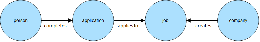
Assume that the goal is to find information about a known job and a known person. Specifically, the idea would be to extract the known job, the company that created the job, the date it was created by the company and whether or not the known person completed an application.
gremlin> g.addV("person").property("name", "bob").as("bob").
           addV("person").property("name", "stephen").as("stephen").
           addV("company").property("name", "Blueprints, Inc").as("blueprints").
           addV("company").property("name", "Rexster, LLC").as("rexster").
           addV("job").property("name", "job1").as("blueprintsJob1").
           addV("job").property("name", "job2").as("blueprintsJob2").
           addV("job").property("name", "job3").as("blueprintsJob3").
           addV("job").property("name", "job4").as("rexsterJob1").
           addV("application").property("name", "application1").as("appBob1").
           addV("application").property("name", "application2").as("appBob2").
           addV("application").property("name", "application3").as("appStephen1").
           addV("application").property("name", "application4").as("appStephen2").
           addE("completes").from("bob").to("appBob1").
           addE("completes").from("bob").to("appBob2").
           addE("completes").from("stephen").to("appStephen1").
           addE("completes").from("stephen").to("appStephen2").
           addE("appliesTo").from("appBob1").to("blueprintsJob1").
           addE("appliesTo").from("appBob2").to("blueprintsJob2").
           addE("appliesTo").from("appStephen1").to("rexsterJob1").
           addE("appliesTo").from("appStephen2").to("blueprintsJob3").
           addE("created").from("blueprints").to("blueprintsJob1").property("creationDate", "12/20/2015").
           addE("created").from("blueprints").to("blueprintsJob2").property("creationDate", "12/15/2015").
           addE("created").from("blueprints").to("blueprintsJob3").property("creationDate", "12/16/2015").
           addE("created").from("rexster").to("rexsterJob1").property("creationDate", "12/18/2015").iterate()
gremlin> vBlueprintsJob1 = g.V().has("job", "name", "job1").next()
==>v[8]
gremlin> vRexsterJob1 = g.V().has("job", "name", "job4").next()
==>v[14]
gremlin> vStephen = g.V().has("person", "name", "stephen").next()
==>v[2]
gremlin> vBob = g.V().has("person", "name", "bob").next()
==>v[0]
gremlin> g.V(vRexsterJob1).as('job').
           inE('created').as('created').
           outV().as('company').
           select('job').
           coalesce(__.in('appliesTo').where(__.in('completes').is(vStephen)),
                    constant(false)).as('application').
           select('job', 'company', 'created', 'application').
             by().by().by('creationDate').by()
==>[job:v[14],company:v[6],created:12/18/2015,application:v[20]]
gremlin> g.V(vRexsterJob1, vBlueprintsJob1).as('job').
           inE('created').as('created').
           outV().as('company').
           select('job').
           coalesce(__.in('appliesTo').where(__.in('completes').is(vBob)),
                    constant(false)).as('application').
           select('job', 'company', 'created', 'application').
             by().by().by('creationDate').by()
==>[job:v[14],company:v[6],created:12/18/2015,application:false]
==>[job:v[8],company:v[4],created:12/20/2015,application:v[16]]
While the traversals above are more complex, the pattern for finding "things" between two vertices is largely the same.
Note the use of the where() step to terminate the traversers for a specific user. It is embedded in a coalesce()
step to handle situations where the specified user did not complete an application for the specified job and will
return false in those cases.
Centrality
There are many measures of centrality which are meant to help identify the most important vertices in a graph. As these measures are common in graph theory, this section attempts to demonstrate how some of these different indicators can be calculated using Gremlin.
Degree Centrality
Degree centrality is a measure of the number of edges associated to each vertex. The following examples use the modern toy graph:
gremlin> g.V().group().by().by(bothE().count()) //1\
==>[v[1]:3,v[2]:1,v[3]:3,v[4]:3,v[5]:1,v[6]:1]
gremlin> g.V().group().by().by(inE().count()) //2\
==>[v[1]:0,v[2]:1,v[3]:3,v[4]:1,v[5]:1,v[6]:0]
gremlin> g.V().group().by().by(outE().count()) //3\
==>[v[1]:3,v[2]:0,v[3]:0,v[4]:2,v[5]:0,v[6]:1]
gremlin> g.V().project("v","degree").by().by(bothE().count()) //4\
==>[v:v[1],degree:3]
==>[v:v[2],degree:1]
==>[v:v[3],degree:3]
==>[v:v[4],degree:3]
==>[v:v[5],degree:1]
==>[v:v[6],degree:1]
gremlin> g.V().project("v","degree").by().by(bothE().count()). //5\
           order().by(select("degree"), decr).
           limit(4)
==>[v:v[1],degree:3]
==>[v:v[3],degree:3]
==>[v:v[4],degree:3]
==>[v:v[2],degree:1]-
Calculation of degree centrality which counts all incident edges on each vertex to include those that are both incoming and outgoing.
-
Calculation of in-degree centrality which only counts incoming edges to a vertex.
-
Calculation of out-degree centrality which only counts outgoing edges from a vertex.
-
The previous examples all produce a single
Mapas their output. While that is a desirable output, producing a stream ofMapobjects can allow some greater flexibility. -
For example, use of a stream enables use of an ordered limit that can be executed in a distributed fashion in OLAP traversals.
|
Note
|
The group step takes up to two separate
by modulators. The first by() tells group()
what the key in the resulting Map will be (i.e. the value to group on). In the above examples, the by() is empty
and as a result, the grouping will be on the incoming Vertex object itself. The second by() is the value to be
stored in the Map for each key.
|
Betweeness Centrality
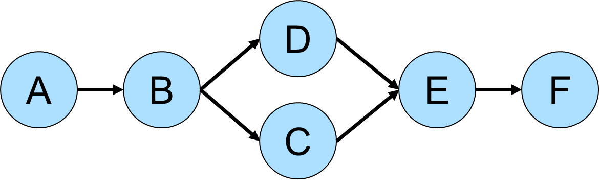
Betweeness centrality is a measure of the number of times a vertex is found between the shortest path of each vertex pair in a graph. Consider the following graph for demonstration purposes:
gremlin> g.addV().property(id,'A').as('a').
           addV().property(id,'B').as('b').
           addV().property(id,'C').as('c').
           addV().property(id,'D').as('d').
           addV().property(id,'E').as('e').
           addV().property(id,'F').as('f').
           addE('next').from('a').to('b').
           addE('next').from('b').to('c').
           addE('next').from('b').to('d').
           addE('next').from('c').to('e').
           addE('next').from('d').to('e').
           addE('next').from('e').to('f').iterate()
gremlin> g.V().as("v"). //1\
           repeat(both().simplePath().as("v")).emit(). //2\
           filter(project("x","y","z").by(select(first, "v")). //3\
                                       by(select(last, "v")).
                                       by(select(all, "v").count(local)).as("triple").
                  coalesce(select("x","y").as("a"). //4\
                             select("triples").unfold().as("t").
                             select("x","y").where(eq("a")).
                             select("t"),
                           store("triples")). //5\
                  select("z").as("length").
                  select("triple").select("z").where(eq("length"))). //6\
           select(all, "v").unfold(). //7\
           groupCount().next() //8\
==>v[A]=14
==>v[B]=28
==>v[C]=20
==>v[D]=20
==>v[E]=28
==>v[F]=14-
Starting from each vertex in the graph…
-
…traverse on both - incoming and outgoing - edges, avoiding cyclic paths.
-
Create a triple consisting of the first vertex, the last vertex and the length of the path between them.
-
Determine whether a path between those two vertices was already found.
-
If this is the first path between the two vertices, store the triple in an internal collection named "triples".
-
Keep only those paths between a pair of vertices that have the same length as the first path that was found between them.
-
Select all shortest paths and unfold them.
-
Count the number of occurrences of each vertex, which is ultimately its betweeness score.
|
Warning
|
Since the betweeness centrality algorithm requires the shortest path between any pair of vertices in the graph, its practical applications are very limited. It’s recommended to use this algorithm only on small subgraphs (graphs like the Grateful Dead graph with only 808 vertices and 8049 edges already require a massive amount of compute resources to determine the shortest paths between all vertex pairs). |
Closeness Centrality
Closeness centrality is a measure of the distance of one vertex to all other reachable vertices in the graph. The following examples use the modern toy graph:
gremlin> g = TinkerFactory.createModern().traversal()
==>graphtraversalsource[tinkergraph[vertices:6 edges:6], standard]
gremlin> g.withSack(1f).V().as("v"). //1\
           repeat(both().simplePath().as("v")).emit(). //2\
           filter(project("x","y","z").by(select(first, "v")). //3\
                                       by(select(last, "v")).
                                       by(select(all, "v").count(local)).as("triple").
                  coalesce(select("x","y").as("a"). //4\
                             select("triples").unfold().as("t").
                             select("x","y").where(eq("a")).
                             select("t"),
                           store("triples")). //5\
                  select("z").as("length").
                  select("triple").select("z").where(eq("length"))). //6\
           group().by(select(first, "v")). //7\
                   by(select(all, "v").count(local).sack(div).sack().sum()).next()
==>v[1]=2.1666666666666665
==>v[2]=1.6666666666666665
==>v[3]=2.1666666666666665
==>v[4]=2.1666666666666665
==>v[5]=1.6666666666666665
==>v[6]=1.6666666666666665-
Defines a Gremlin sack with a value of one.
-
Traverses on both - incoming and outgoing - edges, avoiding cyclic paths.
-
Create a triple consisting of the first vertex, the last vertex and the length of the path between them.
-
Determine whether a path between those two vertices was already found.
-
If this is the first path between the two vertices, store the triple in an internal collection named "triples".
-
Keep only those paths between a pair of vertices that have the same length as the first path that was found between them.
-
For each vertex divide 1 by the product of the lengths of all shortest paths that start with this particular vertex.
|
Warning
|
Since the closeness centrality algorithm requires the shortest path between any pair of vertices in the graph, its practical applications are very limited. It’s recommended to use this algorithm only on small subgraphs (graphs like the Grateful Dead graph with only 808 vertices and 8049 edges already require a massive amount of compute resources to determine the shortest paths between all vertex pairs). |
Eigenvector Centrality
A calculation of eigenvector centrality uses the relative importance of adjacent vertices to help determine their centrality. In other words, unlike degree centrality the vertex with the greatest number of incident edges does not necessarily give it the highest rank. Consider the following example using the Grateful Dead graph:
gremlin> graph.io(graphml()).readGraph('data/grateful-dead.xml')
gremlin> g.V().repeat(groupCount('m').by('name').out()).times(5).cap('m'). //1\
           order(local).by(values, decr).limit(local, 10).next() //2\
==>PLAYING IN THE BAND=8758598
==>ME AND MY UNCLE=8214246
==>JACK STRAW=8173882
==>EL PASO=7666994
==>TRUCKING=7643494
==>PROMISED LAND=7339027
==>CHINA CAT SUNFLOWER=7322213
==>CUMBERLAND BLUES=6730838
==>RAMBLE ON ROSE=6676667
==>LOOKS LIKE RAIN=6674121
gremlin> g.V().repeat(groupCount('m').by('name').out().timeLimit(100)).times(5).cap('m'). //3\
           order(local).by(values, decr).limit(local, 10).next()
==>PLAYING IN THE BAND=8758598
==>ME AND MY UNCLE=8214246
==>JACK STRAW=8173882
==>EL PASO=7666994
==>TRUCKING=7643494
==>PROMISED LAND=7339027
==>CHINA CAT SUNFLOWER=7322213
==>CUMBERLAND BLUES=6730838
==>RAMBLE ON ROSE=6676667
==>LOOKS LIKE RAIN=6674121-
The traversal iterates through each vertex in the graph and for each one repeatedly group counts each vertex that passes through using the vertex as the key. The
Mapof this group count is stored in a variable named "m". Theout()traversal is repeated thirty times or until the paths are exhausted. Five iterations should provide enough time to converge on a solution. Callingcap('m')at the end simply extracts theMapside-effect stored in "m". -
The entries in the
Mapare then iterated and sorted with the top ten most central vertices presented as output. -
The previous examples can be expanded on a little bit by including a time limit. The
timeLimit()prevents the traversal from taking longer than one hundred milliseconds to execute (the previous example takes considerably longer than that). While the answer provided with thetimeLimit()is not the absolute ranking, it does provide a relative ranking that closely matches the absolute one. The use oftimeLimit()in certain algorithms (e.g. recommendations) can shorten the time required to get a reasonable and usable result.
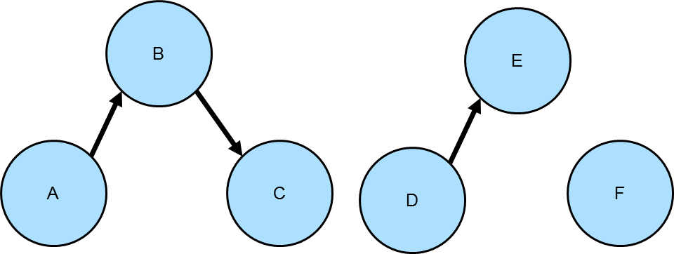
Connected Components
Gremlin can be used to find connected components in a graph. Consider the following graph which has three connected components:
gremlin> g.addV().property(id, "A").as("a").
           addV().property(id, "B").as("b").
           addV().property(id, "C").as("c").
           addV().property(id, "D").as("d").
           addV().property(id, "E").as("e").
           addV().property(id, "F").
           addE("link").from("a").to("b").
           addE("link").from("b").to("c").
           addE("link").from("d").to("e").iterate()
One way to detect the various subgraphs would be to do something like this:
gremlin> g.V().emit(cyclicPath().or().not(both())).repeat(both()).until(cyclicPath()). //1\
           path().aggregate("p"). //2\
           unfold().dedup(). //3\
           map(__.as("v").select("p").unfold(). //4\
                  filter(unfold().where(eq("v"))).
                  unfold().dedup().order().by(id).fold()).
           dedup() //5\
==>[v[A],v[B],v[C]]
==>[v[D],v[E]]
==>[v[F]]-
Iterate all vertices and repeatedly traverse over both incoming and outgoing edges (TinkerPop doesn’t support unidirectional graphs directly so it must be simulated by ignoring the direction with
both). Note the use ofemitprior torepeatas this allows for return of a single length path. -
Aggregate the
path()of the emitted vertices to "p". It is within these paths that the list of connected components will be identified. Obviously the paths list are duplicative in the sense that they contains different paths traveled over the same vertices. -
Unroll the elements in the path list with
unfoldanddedup. -
Use the first vertex in each path to filter against the paths stored in "p". When a path is found that has the vertex in it, dedup the vertices in the path, order it by the identifier. Each path output from this
mapstep represents a connected component. -
The connected component list is duplicative given the nature of the paths in "p", but now that the vertices within the paths are ordered, a final
dedupwill make the list of connective components unique.
|
Note
|
This is a nice example of where running smaller pieces of a large Gremlin statement make it easier to see what is happening at each step. Consider running this example one line at a time (or perhaps even in a step at a time) to see the output at each point. |
While the above approach returns results nicely, the traversal doesn’t appear to work with OLAP. A less efficient
approach, but one more suited for OLAP execution looks quite similar but does not use dedup as heavily (thus
GraphComputer is forced to analyze far more paths):
gremlin> g.withComputer().V().emit(cyclicPath().or().not(both())).repeat(both()).until(cyclicPath()).
aggregate("p").by(path()).cap("p").unfold().limit(local, 1).
map(__.as("v").select("p").unfold().
filter(unfold().where(eq("v"))).
unfold().dedup().order().by(id).fold()
).toSet()
==>[v[A],v[B],v[C]]
==>[v[D],v[E]]
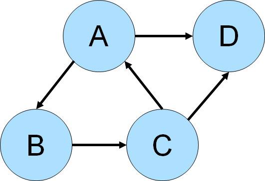
==>[v[F]]Cycle Detection
A cycle occurs in a graph where a path loops back on itself to the originating vertex. For example, in the graph
depicted below Gremlin could be use to detect the cycle among vertices A-B-C.
gremlin> g.addV().property(id,'a').as('a').
           addV().property(id,'b').as('b').
           addV().property(id,'c').as('c').
           addV().property(id,'d').as('d').
           addE('knows').from('a').to('b').
           addE('knows').from('b').to('c').
           addE('knows').from('c').to('a').
           addE('knows').from('a').to('d').
           addE('knows').from('c').to('d').iterate()
gremlin> g.V().as('a').repeat(out().simplePath()).times(2).
           where(out().as('a')).path() //1\
==>[v[a],v[b],v[c]]
==>[v[b],v[c],v[a]]
==>[v[c],v[a],v[b]]
gremlin> g.V().as('a').repeat(out().simplePath()).times(2).
           where(out().as('a')).path().
           dedup().by(unfold().order().by(id).dedup().fold()) //2\
==>[v[a],v[b],v[c]]-
Gremlin starts its traversal from a vertex labeled "a" and traverses
out()from each vertex filtering on thesimplePath, which removes paths with repeated objects. The steps goingout()are repeated twice as in this case the length of the cycle is known to be three and there is no need to exceed that. The traversal filters with awhere()to see only return paths that end with where it started at "a". -
The previous query returned the
A-B-Ccycle, but it returned three paths which were all technically the same cycle. It returned three, because there was one for each vertex that started the cycle (i.e. one forA, one forBand one forC). This next line introduce deduplication to only return unique cycles.
The above case assumed that the need was to only detect cycles over a path length of three. It also respected the directionality of the edges by only considering outgoing ones. What would need to change to detect cycles of arbitrary length over both incoming and outgoing edges in the modern graph?
gremlin> g.V().as('a').repeat(both().simplePath()).emit(loops().is(gt(1))).
           both().where(eq('a')).path().
           dedup().by(unfold().order().by(id).dedup().fold())
==>[v[1],v[3],v[4],v[1]]
An interesting type of cycle is known as the Eulerian circuit which is a path taken in a graph where each edge is visited once and the path starts and ends with the same vertex. Consider the following graph, representative of an imaginary but geographically similar Königsberg that happens to have an eighth bridge (the diagram depicts edge direction but direction won’t be considered in the traversal):
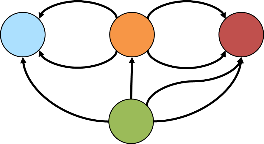
Gremlin can detect if such a cycle exists with:
gremlin> g.addV().property(id, 'blue').as('b').
           addV().property(id, 'orange').as('o').
           addV().property(id, 'red').as('r').
           addV().property(id, 'green').as('g').
           addE('bridge').from('g').to('b').
           addE('bridge').from('g').to('o').
           addE('bridge').from('g').to('r').
           addE('bridge').from('g').to('r').
           addE('bridge').from('o').to('b').
           addE('bridge').from('o').to('b').
           addE('bridge').from('o').to('r').
           addE('bridge').from('o').to('r').iterate()
gremlin> g.V().sideEffect(outE("bridge").aggregate("bridges")).barrier(). //1\
           repeat(bothE(). //2\
                  or(__.not(select('e')),
                     __.not(filter(__.as('x').select(all, 'e').unfold(). //3\
                            where(eq('x'))))).as('e').
                  otherV()).
             until(select(all, 'e').count(local).as("c"). //4\
                   select("bridges").count(local).where(eq("c"))).hasNext()
==>true-
Gather all the edges in a "bridges" side effect.
-
As mentioned earlier with the diagram, directionality is ignored as the traversal uses
bothEand, later,otherV. -
In continually traversing over both incoming and outgoing edges, this path is only worth continuing if the edges traversed thus far are only traversed once. That set of edges is maintained in "e".
-
The traversal should repeat until the number of edges traversed in "e" is equal to the total number gathered in the first step above, which would mean that the complete circuit has been made.
Unlike Königsberg, with just seven bridges, a Eulerian circuit exists in the case with an eighth bridge. The first detected circuit can be displayed with:
gremlin> g.V().sideEffect(outE("bridge").aggregate("bridges")).barrier().
           repeat(bothE().or(__.not(select('e')),
                             __.not(filter(__.as('x').select(all, 'e').unfold().
                                    where(eq('x'))))).as('e').otherV()).
             until(select(all, 'e').count(local).as("c").
                   select("bridges").count(local).where(eq("c"))).limit(1).
           path().by(id).by(constant(" -> ")).
           map {String.join("", it.get().objects())}
==>orange -> blue -> green -> orange -> red -> green -> red -> orange -> blue
Duplicate Edge Detection
Whether part of a graph maintenance process or for some other analysis need, it is sometimes necessary to detect if there is more than one edge between two vertices. The following examples will assume that an edge with the same label and direction will be considered "duplicate".
The "modern" graph does not have any duplicate edges that fit that definition, so the following example adds one that is duplicative of the "created" edge between vertex "1" and "3".
gremlin> g.V(1).as("a").V(3).addE("created").from("a").iterate()
gremlin> g.V(1).outE("created")
==>e[9][1-created->3]
==>e[13][1-created->3]
One way to find the duplicate edges would be to do something like this:
gremlin> g.V().outE().
           project("a","b"). //1\
             by().by(inV().path().by().by(label)).
           group(). //2\
             by(select("b")).
             by(select("a").fold()).
           unfold(). //3\
           select(values). //4\
           where(count(local).is(gt(1)))
==>[e[9][1-created->3],e[13][1-created->3]]-
The "a" and "b" from the
projectcontain the edge and the path respectively. The path consists of a the outgoing vertex, an edge, and the incoming vertex. The use ofby().by(label))converts the edge to its label (recall thatbyare applied in round-robin fashion), so the path will look something like:[v[1],created,v[3]]. -
Group by the path from "b" and construct a list of edges from "a". Any value in this
Mapthat has a list of edges greater than one means that there is more than one edge for that edge label between those two vertices (i.e. theMapkey). -
Unroll the key-value pairs in the
Mapof paths-edges. -
Only the values from the
Mapare needed and as mentioned earlier, those lists with more than one edge would contain duplicate.
This method find the duplicates, but does require more memory than other approaches. A slightly more complex approach that uses less memory might look like this:
gremlin> g.V().as("ov").
           outE().as("e").
           inV().as("iv").
           inE(). //1\
           where(neq("e")). //2\
           where(eq("e")).by(label).
           where(outV().as("ov")).
           group().
             by(select("ov","e","iv").by().by(label)). //3\
           unfold(). //4\
           select(values).
           where(count(local).is(gt(1)))
==>[e[13][1-created->3],e[9][1-created->3]]-
To this point in the traversal, the outgoing edges of a vertex are being iterated with the current edge labeled as "e". For "e", Gremlin traverses to the incoming vertex and back on in edges of that vertex.
-
Those incoming edges are filtered with the following
wheresteps. The first ensures that it does not traverse back over "e" (i.e. the current edge). The second determines if the edge label is equivalent (i.e. the test for the working definition of "duplicate"). The third determines if the outgoing vertex matches the one that started the path labeled as "ov". -
This line is quite similar to the output achieved in the previous example at step 2. A
Mapis produced that uses the outgoing vertex, the edge label, and the incoming vertex as the key, with the list of edges for that path as the value. -
The rest of the traversal is the same as the previous one.
Note that the above traversal could also be written using match step:
gremlin> g.V().match(
             __.as("ov").outE().as("e"),
             __.as("e").inV().as("iv"),
             __.as("iv").inE().as("ie"),
             __.as("ie").outV().as("ov")).
               where("ie",neq("e")).
               where("ie",eq("e")).by(label).
             select("ie").
             group().
               by(select("ov","e","iv").by().by(label)).
             unfold().select(values).
               where(count(local).is(gt(1)))
==>[e[13][1-created->3],e[9][1-created->3]]
A third way to approach this problem would be to force a depth-first search. The previous examples invoke traversal strategies that force a breadth first search as a performance optimization.
gremlin> g.withoutStrategies(LazyBarrierStrategy, PathRetractionStrategy).V().as("ov"). //1\
           outE().as("e1").
           inV().as("iv").
           inE().
           where(neq("e1")).
           where(outV().as("ov")).as("e2"). //2\
           where("e1", eq("e2")).by(label) //3\
==>e[13][1-created->3]
==>e[9][1-created->3]-
Remove strategies that will optimize for breadth first searches and thus allow Gremlin to go depth first.
-
To this point, the traversal is very much like the previous one. Review step 2 in the previous example to see the parallels here.
-
The final
wheresimply looks for edges that match on label, which would then meet the working definition of "duplicate".
The basic pattern at play here is to compare the path of the outgoing vertex, its outgoing edge label and the incoming vertex. This model can obviously be contracted or expanded as needed to fit different definitions of "duplicate". For example, a "duplicate" definition could extended to the label and properties of the edge. For purposes of demonstration, an additional edge is added to the "modern" graph:
gremlin> g.V(1).as("a").V(3).addE("created").property("weight",0.4d).from("a").iterate()
gremlin> g.V(1).as("a").V(3).addE("created").property("weight",0.5d).from("a").iterate()
gremlin> g.V(1).outE("created").valueMap(true)
==>[id:9,weight:0.4,label:created]
==>[id:13,weight:0.4,label:created]
==>[id:14,weight:0.5,label:created]
To identify the duplicate with this revised definition, the previous traversal can be modified to:
gremlin> g.withoutStrategies(LazyBarrierStrategy, PathRetractionStrategy).V().as("ov").
           outE().as("e1").
           inV().as("iv").
           inE().
           where(neq("e1")).
           where(outV().as("ov")).as("e2").
           where("e1", eq("e2")).by(label).
           where("e1", eq("e2")).by("weight").valueMap(true)
==>[id:13,weight:0.4,label:created]
==>[id:9,weight:0.4,label:created]
Duplicate Vertex Detection
The pattern for finding duplicate vertices is quite similar to the pattern defined in the Duplicate Edge section. The idea is to extract the relevant features of the vertex into a comparable list that can then be used to group for duplicates.
Consider the following example with some duplicate vertices added to the "modern" graph:
gremlin> g.addV('person').property('name', 'vadas').property('age', 27)
==>v[13]
gremlin> g.addV('person').property('name', 'vadas').property('age', 22) // not a duplicate because "age" value
==>v[16]
gremlin> g.addV('person').property('name', 'marko').property('age', 29)
==>v[19]
gremlin> g.V().hasLabel("person").
           group().
             by(values("name", "age").fold()).
           unfold()
==>[marko, 29]=[v[1], v[19]]
==>[vadas, 27]=[v[2], v[13]]
==>[peter, 35]=[v[6]]
==>[vadas, 22]=[v[16]]
==>[josh, 32]=[v[4]]
In the above case, the "name" and "age" properties are the relevant features for identifying duplication. The key in
the Map provided by the group is the list of features for comparison and the value is the list of vertices that
match the feature. To extract just those vertices that contain duplicates an additional filter can be added:
gremlin> g.V().hasLabel("person").
           group().
             by(values("name", "age").fold()).
           unfold().
           filter(select(values).count(local).is(gt(1)))
==>[marko, 29]=[v[1], v[19]]
==>[vadas, 27]=[v[2], v[13]]
That filter, extracts the values of the Map and counts the vertices within each list. If that list contains more than
one vertex then it is a duplicate.
If-Then Based Grouping
Consider the following traversal over the "modern" toy graph:
gremlin> g.V().hasLabel('person').groupCount().by('age')
==>[32:1,35:1,27:1,29:1]
The result is an age distribution that simply shows that every "person" in the graph is of a different age. In some cases, this result is exactly what is needed, but sometimes a grouping may need to be transformed to provide a different picture of the result. For example, perhaps a grouping on the value "age" would be better represented by a domain concept such as "young", "old" and "very old".
gremlin> g.V().hasLabel("person").groupCount().by(values("age").choose(
           is(lt(28)),constant("young"),
           choose(is(lt(30)),
                  constant("old"),
                  constant("very old"))))
==>[young:1,old:1,very old:2]
Note that the by modulator has been altered from simply taking a string key of "age" to take a Traversal. That
inner Traversal utilizes choose which is like an if-then-else clause. The choose is nested and would look
like the following in Java:
if (age < 28) {
  return "young";
} else {
  if (age < 30) {
    return "old";
  } else {
    return "very old";
  }
}
The use of choose is a good intuitive choice for this Traversal as it is a natural mapping to if-then-else, but
there is another option to consider with coalesce:
gremlin> g.V().hasLabel("person").
           groupCount().by(values("age").
           coalesce(is(lt(28)).constant("young"),
                    is(lt(30)).constant("old"),
                    constant("very old")))
==>[young:1,old:1,very old:2]
The answer is the same, but this traversal removes the nested choose, which makes it easier to read.
Pagination
 In most database applications, it is oftentimes desirable to return
discrete blocks of data for a query rather than all of the data that the total results would contain. This approach to
returning data is referred to as "pagination" and typically involves a situation where the client executing the query
can specify the start position and end position (or the amount of data to return in lieu of the end position)
representing the block of data to return. In this way, one could return the first ten records of one hundred, then the
second ten records and so on, until potentially all one hundred were returned.
In most database applications, it is oftentimes desirable to return
discrete blocks of data for a query rather than all of the data that the total results would contain. This approach to
returning data is referred to as "pagination" and typically involves a situation where the client executing the query
can specify the start position and end position (or the amount of data to return in lieu of the end position)
representing the block of data to return. In this way, one could return the first ten records of one hundred, then the
second ten records and so on, until potentially all one hundred were returned.
In Gremlin, a basic approach to paging would look something like the following:
gremlin> g.V().hasLabel('person').fold() //1\
==>[v[1],v[2],v[4],v[6]]
gremlin> g.V().hasLabel('person').
           fold().as('persons','count').
           select('persons','count').
             by(range(local, 0, 2)).
             by(count(local)) //2\
==>[persons:[v[1],v[2]],count:4]
gremlin> g.V().hasLabel('person').
           fold().as('persons','count').
           select('persons','count').
             by(range(local, 2, 4)).
             by(count(local)) //3\
==>[persons:[v[4],v[6]],count:4]-
Gets all the "person" vertices.
-
Gets the first two "person" vertices and includes the total number of vertices so that the client knows how many it has to page through.
-
Gets the final two "person" vertices.
From a functional perspective, the above example shows a fairly standard paging model. Unfortunately, there is a
problem. To get the total number of vertices, the traversal must first fold() them, which iterates out
the traversal bringing them all into memory. If the number of "person" vertices is large, that step could lead to a
long running traversal and perhaps one that would simply run out of memory prior to completion. There is no shortcut
to getting a total count without doing a full iteration of the traversal. If the requirement for a total count is
removed then the traversals become more simple:
gremlin> g.V().hasLabel('person').range(0,2)
==>v[1]
==>v[2]
gremlin> g.V().hasLabel('person').range(2,4)
==>v[4]
==>v[6]|
Note
|
The first traversal above could also be written as g.V().hasLabel('person').limit(2).
|
In this case, there is no way to know the total count so the only way to know if the end of the results have been
reached is to count the results from each paged result to see if there’s less than the number expected or simply zero
results. In that case, further requests for additional pages would be unnecessary. Of course, this approach is not
free of problems either. Most graph databases will not optimize the range() step, meaning that the second traversal
will repeat the iteration of the first two vertices to get to the second set of two vertices. In other words, for the
second traversal, the graph will still read four vertices even though there was only a request for two.
The only way to completely avoid that problem is to re-use the same traversal instance:
gremlin> t = g.V().hasLabel('person');[]
gremlin> t.next(2)
==>v[1]
==>v[2]
gremlin> t.next(2)
==>v[4]
==>v[6]
Recommendation
 One of the more common use cases for a graph database is the
development of recommendation systems and a simple approach to
doing that is through collaborative filtering.
Collaborative filtering assumes that if a person shares one set of opinions with a different person, they are likely to
have similar taste with respect to other issues. With that basis in mind, it is then possible to make predictions for a
specific person as to what their opinions might be.
One of the more common use cases for a graph database is the
development of recommendation systems and a simple approach to
doing that is through collaborative filtering.
Collaborative filtering assumes that if a person shares one set of opinions with a different person, they are likely to
have similar taste with respect to other issues. With that basis in mind, it is then possible to make predictions for a
specific person as to what their opinions might be.
As a simple example, consider a graph that contains "person" and "product" vertices connected by "bought" edges. The following script generates some data for the graph using that basic schema:
gremlin> g.addV("person").property("name","alice").
           addV("person").property("name","bob").
           addV("person").property("name","jon").
           addV("person").property("name","jack").
           addV("person").property("name","jill")iterate()
gremlin> (1..10).each {
           g.addV("product").property("name","product #${it}").iterate()
         }; []
gremlin> (3..7).each {
           g.V().has("person","name","alice").as("p").
             V().has("product","name","product #${it}").addE("bought").from("p").iterate()
         }; []
gremlin> (1..5).each {
           g.V().has("person","name","bob").as("p").
             V().has("product","name","product #${it}").addE("bought").from("p").iterate()
         }; []
gremlin> (6..10).each {
           g.V().has("person","name","jon").as("p").
             V().has("product","name","product #${it}").addE("bought").from("p").iterate()
         }; []
gremlin> 1.step(10, 2) {
           g.V().has("person","name","jack").as("p").
             V().has("product","name","product #${it}").addE("bought").from("p").iterate()
         }; []
gremlin> 2.step(10, 2) {
           g.V().has("person","name","jill").as("p").
             V().has("product","name","product #${it}").addE("bought").from("p").iterate()
         }; []
The first step to making a recommendation to "alice" using collaborative filtering is to understand what she bought:
gremlin> g.V().has('name','alice').out('bought').values('name')
==>product #5
==>product #6
==>product #7
==>product #3
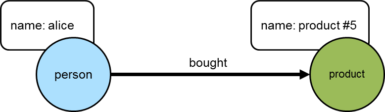
==>product #4The following diagram depicts one of the edges traversed in the above example between "alice" and "product #5". Obviously, the other products "alice" bought would have similar relations, but this diagram and those to follow will focus on the neighborhood around that product.
The next step is to determine who else purchased those products:
gremlin> g.V().has('name','alice').out('bought').in('bought').dedup().values('name')
==>alice
==>bob
==>jack
==>jill
==>jon
It is worth noting that "alice" is in the results above. She should really be excluded from the list as the interest is in what individuals other than herself purchased:
gremlin> g.V().has('name','alice').as('her').
out('bought').
in('bought').where(neq('her')).
dedup().values('name')
==>bob
==>jack
==>jill
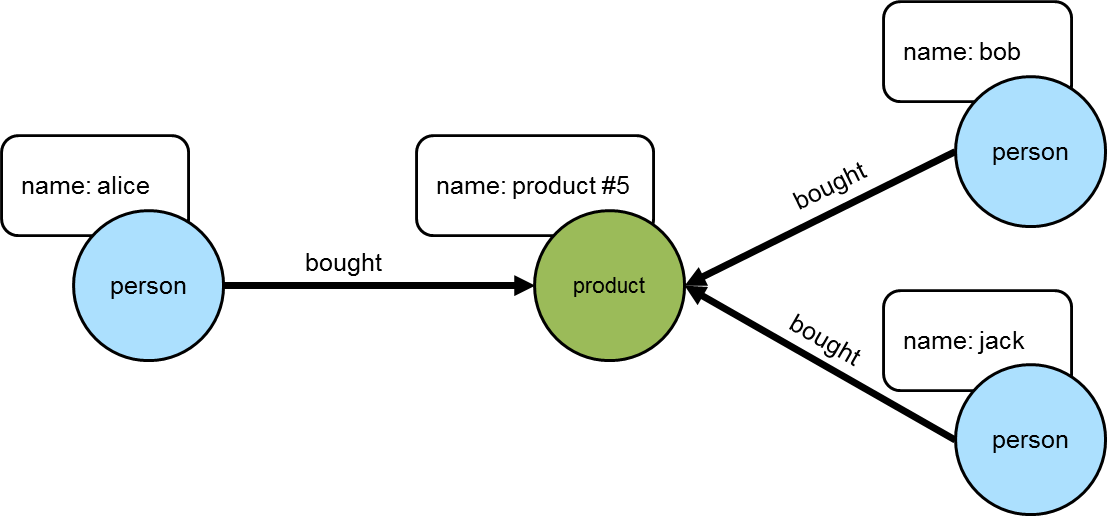
==>jonThe following diagram shows "alice" and those others who purchased "product #5".
The knowledge of the people who bought the same things as "alice" can then be used to find the set of products that they bought:
gremlin> g.V().has('name','alice').as('her').
               out('bought').
               in('bought').where(neq('her')).
               out('bought').
               dedup().values('name')
==>product #1
==>product #2
==>product #3
==>product #4
==>product #5
==>product #7
==>product #9
==>product #6
==>product #8
==>product #10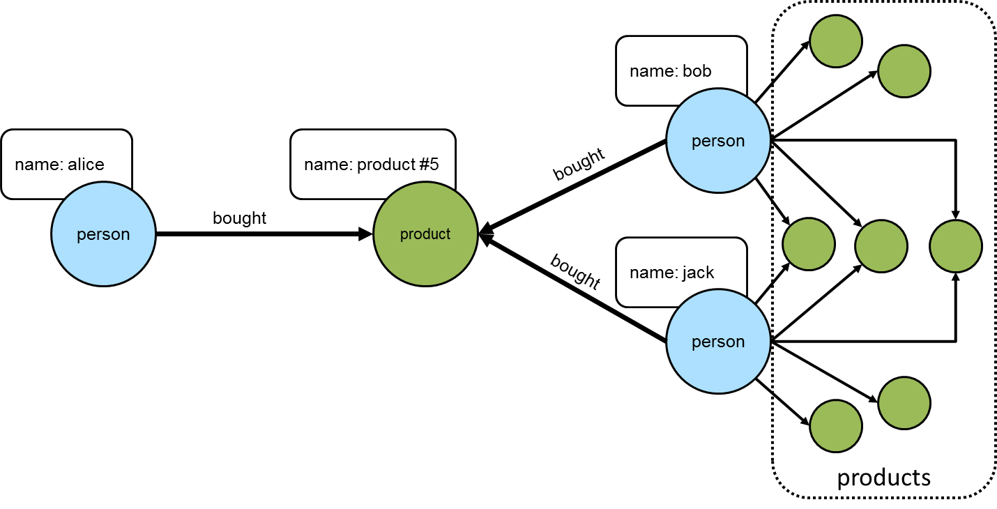
This set of products could be the basis for recommendation, but it is important to remember that "alice" may have already purchased some of these products and it would be better to not pester her with recommendations for products that she already owns. Those products she already purchased can be excluded as follows:
gremlin> g.V().has('name','alice').as('her').
               out('bought').aggregate('self').
               in('bought').where(neq('her')).
               out('bought').where(without('self')).
               dedup().values('name')
==>product #1
==>product #2
==>product #9
==>product #8
==>product #10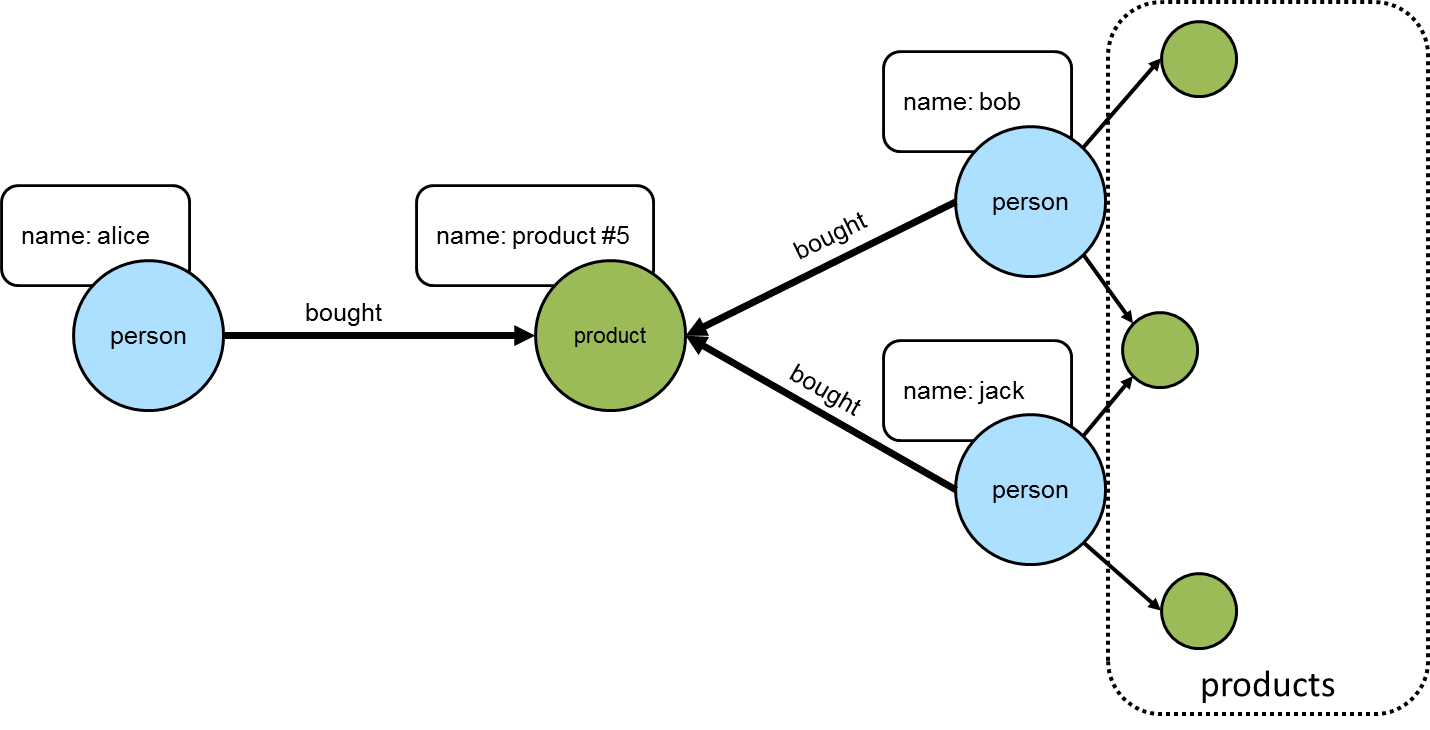
The final step would be to group the remaining products (instead of dedup() which was mostly done for demonstration
purposes) to form a ranking:
gremlin> g.V().has('person','name','alice').as('her'). //1\
               out('bought').aggregate('self'). //2\
               in('bought').where(neq('her')). //3\
               out('bought').where(without('self')). //4\
               groupCount().
               order(local).
                 by(values, decr) //5\
==>[v[10]:6,v[26]:5,v[12]:5,v[24]:4,v[28]:2]-
Find "alice" who is the person for whom the product recommendation is being made.
-
Traverse to the products that "alice" bought and gather them for later use in the traversal.
-
Traverse to the "person" vertices who bought the products that "alice" bought and exclude "alice" herself from that list.
-
Given those people who bought similar products to "alice", find the products that they bought and exclude those that she already bought.
-
Group the products and count the number of times they were purchased by others to come up with a ranking of products to recommend to "alice".
The previous example was already described as "basic" and obviously could take into account whatever data is available to further improve the quality of the recommendation (e.g. product ratings, times of purchase, etc.). One option to improve the quality of what is recommended (without expanding the previous dataset) might be to choose the person vertices that make up the recommendation to "alice" who have the largest common set of purchases.
Looking back to the previous code example, consider its more strip down representation that shows those individuals who have at least one product in common:
gremlin> g.V().has("person","name","alice").as("alice").
               out("bought").aggregate("self").
               in("bought").where(neq("alice")).dedup()
==>v[2]
==>v[6]
==>v[8]
==>v[4]
Next, do some grouping to find count how many products they have in common:
gremlin> g.V().has("person","name","alice").as("alice").
               out("bought").aggregate("self").
               in("bought").where(neq("alice")).dedup().
               group().
                 by().by(out("bought").
               where(within("self")).count())
==>[v[2]:3,v[4]:2,v[6]:3,v[8]:2]
The above output shows that the best that can be expected is three common products. The traversal needs to be aware of that maximum:
gremlin> g.V().has("person","name","alice").as("alice").
               out("bought").aggregate("self").
               in("bought").where(neq("alice")).dedup().
               group().
                 by().by(out("bought").
               where(within("self")).count()).
               select(values).
               order(local).
                 by(decr).limit(local, 1)
==>3
With the maximum value available, it can be used to chose those "person" vertices that have the three products in common:
gremlin> g.V().has("person","name","alice").as("alice").
               out("bought").aggregate("self").
               in("bought").where(neq("alice")).dedup().
               group().
                 by().by(out("bought").
               where(within("self")).count()).as("g").
               select(values).
               order(local).
                 by(decr).limit(local, 1).as("m").
               select("g").unfold().
               where(select(values).as("m")).select(keys)
==>v[2]
==>v[6]
Now that there is a list of "person" vertices to base the recommendation on, traverse to the products that they purchased:
gremlin> g.V().has("person","name","alice").as("alice").
               out("bought").aggregate("self").
               in("bought").where(neq("alice")).dedup().
               group().
                 by().by(out("bought").
               where(within("self")).count()).as("g").
               select(values).
               order(local).
                 by(decr).limit(local, 1).as("m").
               select("g").unfold().
               where(select(values).as("m")).select(keys).
               out("bought").where(without("self"))
==>v[10]
==>v[12]
==>v[26]
==>v[10]
The above output shows that one product is held in common making it the top recommendation:
gremlin> g.V().has("person","name","alice").as("alice").
               out("bought").aggregate("self").
               in("bought").where(neq("alice")).dedup().
               group().
                 by().by(out("bought").
               where(within("self")).count()).as("g").
               select(values).
               order(local).
                 by(decr).limit(local, 1).as("m").
               select("g").unfold().
               where(select(values).as("m")).select(keys).
               out("bought").where(without("self")).
               groupCount().
               order(local).
                 by(values, decr).
                 by(select(keys).values("name")).
               unfold().select(keys).values("name")
==>product #1
==>product #2
==>product #9
In considering the practical applications of this recipe, it is worth revisiting the earlier "basic" version of the recommendation algorithm:
gremlin> g.V().has('person','name','alice').as('her').
               out('bought').aggregate('self').
               in('bought').where(neq('her')).
               out('bought').where(without('self')).
               groupCount().
               order(local).
                 by(values, decr)
==>[v[10]:6,v[26]:5,v[12]:5,v[24]:4,v[28]:2]
The above traversal performs a full ranking of items based on all the connected data. That could be a time consuming operation depending on the number of paths being traversed. As it turns out, recommendations don’t need to have perfect knowledge of all data to provide a "pretty good" approximation of a recommendation. It can therefore make sense to place additional limits on the traversal to have it better return more quickly at the expense of examining less data.
Gremlin provides a number of steps that can help with these limits like: coin(), sample(), and timeLimit(). For example, to have the traversal sample the data for no longer than one second, the previous "basic" recommendation could be changed to:
gremlin> g.V().has('person','name','alice').as('her').
               out('bought').aggregate('self').
               in('bought').where(neq('her')).
               out('bought').where(without('self')).timeLimit(1000).
               groupCount().
               order(local).
                 by(values, decr)
==>[v[10]:6,v[26]:5,v[12]:5,v[24]:4,v[28]:2]
In using sampling methods, it is important to consider that the natural ordering of edges in the graph may not produce an ideal sample for the recommendation. For example, if the edges end up being returned oldest first, then the recommendation will be based on the oldest data, which would not be ideal. As with any traversal, it is important to understand the nature of the graph being traversed and the behavior of the underlying graph database to properly achieve the desired outcome.
Shortest Path
When working with a graph, it is often necessary to identify the shortest path between two identified vertices. The following is a simple example that identifies the shortest path between vertex "1" and vertex "5" while traversing over out edges:
gremlin> g.addV().property(id, 1).as('1').
           addV().property(id, 2).as('2').
           addV().property(id, 3).as('3').
           addV().property(id, 4).as('4').
           addV().property(id, 5).as('5').
           addE('knows').from('1').to('2').
           addE('knows').from('2').to('4').
           addE('knows').from('4').to('5').
           addE('knows').from('2').to('3').
           addE('knows').from('3').to('4').iterate()
gremlin> g.V(1).repeat(out().simplePath()).until(hasId(5)).path().limit(1) //1\
==>[v[1],v[2],v[4],v[5]]
gremlin> g.V(1).repeat(out().simplePath()).until(hasId(5)).path().count(local) //2\
==>4
==>5
gremlin> g.V(1).repeat(out().simplePath()).until(hasId(5)).path().
           group().by(count(local)).next() //3\
==>4=[[v[1], v[2], v[4], v[5]]]
==>5=[[v[1], v[2], v[3], v[4], v[5]]]-
The traversal starts at vertex with the identifier of "1" and repeatedly traverses on out edges "until" it finds a vertex with an identifier of "5". The inclusion of
simplePathwithin therepeatis present to filter out repeated paths. The traversal terminates withlimitin this case as the first path returned will be the shortest one. Of course, it is possible for there to be more than one path in the graph of the same length (i.e. two or more paths of length three), but this example is not considering that. -
It might be interesting to know the path lengths for all paths between vertex "1" and "5".
-
Alternatively, one might wish to do a path length distribution over all the paths.
The previous example defines the length of the path by the number of vertices in the path, but the "path" might also be measured by data within the graph itself. The following example use the same graph structure as the previous example, but includes a "weight" on the edges, that will be used to help determine the "cost" of a particular path:
gremlin> g.addV().property(id, 1).as('1').
           addV().property(id, 2).as('2').
           addV().property(id, 3).as('3').
           addV().property(id, 4).as('4').
           addV().property(id, 5).as('5').
           addE('knows').from('1').to('2').property('weight', 1.25).
           addE('knows').from('2').to('4').property('weight', 1.5).
           addE('knows').from('4').to('5').property('weight', 0.25).
           addE('knows').from('2').to('3').property('weight', 0.25).
           addE('knows').from('3').to('4').property('weight', 0.25).iterate()
gremlin> g.V(1).repeat(out().simplePath()).until(hasId(5)).path().
           group().by(count(local)).next() //1\
==>4=[[v[1], v[2], v[4], v[5]]]
==>5=[[v[1], v[2], v[3], v[4], v[5]]]
gremlin> g.V(1).repeat(outE().inV().simplePath()).until(hasId(5)).
           path().by(coalesce(values('weight'),
                              constant(0.0))).
           map(unfold().sum()) //2\
==>3.00
==>2.00
gremlin> g.V(1).repeat(outE().inV().simplePath()).until(hasId(5)).
           path().by(constant(0.0)).by('weight').map(unfold().sum()) //3\
==>3.00
==>2.00
gremlin> g.V(1).repeat(outE().inV().simplePath()).until(hasId(5)).
           path().as('p').
           map(unfold().coalesce(values('weight'),
                                 constant(0.0)).sum()).as('cost').
           select('cost','p') //4\
==>[cost:3.00,p:[v[1],e[0][1-knows->2],v[2],e[1][2-knows->4],v[4],e[2][4-knows->5],v[5]]]
==>[cost:2.00,p:[v[1],e[0][1-knows->2],v[2],e[3][2-knows->3],v[3],e[4][3-knows->4],v[4],e[2][4-knows->5],v[5]]]-
Note that the shortest path as determined by the structure of the graph is the same.
-
Calculate the "cost" of the path as determined by the weight on the edges. As the "weight" data is on the edges between the vertices, it is necessary to change the contents of the
repeatstep to useoutE().inV()so that the edge is included in the path. The path is then post-processed with abymodulator that extracts the "weight" value. The traversal usescoalesceas there is a mixture of vertices and edges in the path and the traversal is only interested in edge elements that can return a "weight" property. The final part of the traversal executes a map function over each path, unfolding it and summing the weights. -
The same traversal as the one above it, but avoids the use of
coalescewith the use of twobymodulators. Thebymodulator is applied in a round-robin fashion, so the firstbywill always apply to a vertex (as it is the first item in every path) and the secondbywill always apply to an edge (as it always follows the vertex in the path). -
The output of the previous examples of the "cost" wasn’t terribly useful as it didn’t include which path had the calculated cost. With some slight modifications given the use of
selectit becomes possible to include the path in the output. Note that the path with the lowest "cost" actually has a longer path length as determined by the graph structure.
Traversal Induced Values
The parameters of a Traversal can be known ahead of time as constants or might otherwise be passed in as dynamic
arguments.
gremlin> g.V().has('name','marko').out('knows').has('age', gt(29)).values('name')
==>josh
In plain language, the above Gremlin asks, "What are the names of the people who Marko knows who are over the age of 29?". In this case, "29" is known as a constant to the traversal. Of course, if the question is changed slightly to instead ask, "What are the names of the people who Marko knows who are older than he is?", the hardcoding of "29" will no longer suffice. There are multiple ways Gremlin would allow this second question to be answered. The first is obvious to any programmer - use a variable:
gremlin> marko = g.V().has('name','marko').next()
==>v[1]
gremlin> g.V(marko).out('knows').has('age', gt(marko.value('age'))).values('name')
==>josh
The downside to this approach is that it takes two separate traversals to answer the question. Ideally, there should
be a single traversal, that can query "marko" once, determine his age and then use that for the value supplied to
filter the people he knows. In this way the value for the age in the has()-filter is induced from the Traversal
itself.
gremlin> g.V().has('name','marko').as('marko'). //1\
           out('knows').as('friend'). //2\
             where('friend', gt('marko')).by('age'). //3\
           values('name') //4\
==>josh-
Find the "marko"
Vertexand label it as "marko". -
Traverse out on the "knows" edges to the adjacent
Vertexand label it as "friend". -
Continue to traverser only if Marko’s current friend is older than him.
-
Get the name of Marko’s older friend.
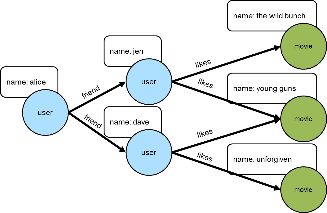
As another example of how traversal induced values can be used, consider a scenario where there was a graph that contained people, their friendship relationships, and the movies that they liked.
gremlin> g.addV("user").property("name", "alice").as("u1").
           addV("user").property("name", "jen").as("u2").
           addV("user").property("name", "dave").as("u3").
           addV("movie").property("name", "the wild bunch").as("m1").
           addV("movie").property("name", "young guns").as("m2").
           addV("movie").property("name", "unforgiven").as("m3").
           addE("friend").from("u1").to("u2").
           addE("friend").from("u1").to("u3").
           addE("like").from("u2").to("m1").
           addE("like").from("u2").to("m2").
           addE("like").from("u3").to("m2").
           addE("like").from("u3").to("m3").iterate()
Getting a list of all the movies that Alice’s friends like could be done like this:
gremlin> g.V().has('name','alice').out("friend").out("like").values("name")
==>the wild bunch
==>young guns
==>young guns
==>unforgiven
but what if there was a need to get a list of movies that all her Alice’s friends liked. In this case, that would mean filtering out "the wild bunch" and "unforgiven".
gremlin> g.V().has("name","alice").
           out("friend").aggregate("friends"). //1\
           out("like").dedup(). //2\
           filter(__.in("like").where(within("friends")).count().as("a"). //3\
                     select("friends").count(local).where(eq("a"))). //4\
           values("name")
==>young guns-
Gather Alice’s list of friends to a list called "friends".
-
Traverse to the unique list of movies that Alice’s friends like.
-
Remove movies that weren’t liked by all friends. This starts by taking each movie and traversing back in on the "like" edges to friends who liked the movie (note the use of
where(within("friends"))to limit those likes to only Alice’s friends as aggregated in step one) and count them up into "a". -
Count the aggregated friends and see if the number matches what was stored in "a" which would mean that all friends like the movie.
Traversal induced values are not just for filtering. They can also be used when writing the values of the properties
of one Vertex to another:
gremlin> g.V().has('name', 'marko').as('marko').
out('created').property('creator', select('marko').by('name'))
==>v[3]
gremlin> g.V().has('name', 'marko').out('created').valueMap()
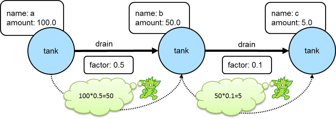
==>[creator:[marko],name:[lop],lang:[java]]In a more complex example of how this might work, consider a situation where the goal is to propagate a value stored on a particular vertex through one of more additional connected vertices using some value on the connecting edges to determine the value to assign. For example, the following graph depicts three "tank" vertices where the edges represent the direction a particular "tank" should drain and the "factor" by which it should do it:
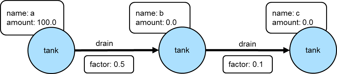
If the traversal started at tank "a", then the value of "amount" on that tank would be used to calculate what the value of tank "b" was by multiplying it by the value of the "factor" property on the edge between vertices "a" and "b". In this case the amount of tank "b" would then be 50. Following this pattern, when going from tank "b" to tank "c", the value of the "amount" of tank "c" would be 5.
Using Gremlin sack(), this kind of operation could be specified as a single traversal:
gremlin> g.addV('tank').property('name', 'a').property('amount', 100.0).as('a').
           addV('tank').property('name', 'b').property('amount', 0.0).as('b').
           addV('tank').property('name', 'c').property('amount', 0.0).as('c').
           addE('drain').property('factor', 0.5).from('a').to('b').
           addE('drain').property('factor', 0.1).from('b').to('c').iterate()
gremlin> a = g.V().has('name','a').next()
==>v[0]
gremlin> g.withSack(a.value('amount')).
           V(a).repeat(outE('drain').sack(mult).by('factor').
                       inV().property('amount', sack())).
                until(__.outE('drain').count().is(0)).iterate()
gremlin> g.V().valueMap()
==>[amount:[100.0],name:[a]]
==>[amount:[50.00],name:[b]]
==>[amount:[5.000],name:[c]]
The "sack value" gets initialized to the value of tank "a". The traversal iteratively traverses out on the "drain"
edges and uses mult to multiply the sack value by the value of "factor". The sack value at that point is then
written to the "amount" of the current vertex.
As shown in the previous example, sack() is a useful way to "carry" and manipulate a value that can be later used
elsewhere in the traversal. Here is another example of its usage where it is utilized to increment all the "age" values
in the modern toy graph by 10:
gremlin> g.withSack(0).V().has("age").
           sack(assign).by("age").sack(sum).by(constant(10)).
           property("age", sack()).valueMap()
==>[name:[marko],age:[39]]
==>[name:[vadas],age:[37]]
==>[name:[josh],age:[42]]
==>[name:[peter],age:[45]]
In the above case, the sack is initialized to zero and as each vertex is iterated, the "age" is assigned to the sack
with sack(assign).by('age'). That value in the sack is then incremented by the value constant(10) and assigned to
the "age" property of the same vertex.
This value the sack is incremented by need not be a constant. It could also be derived from the traversal itself. Using the same example, the "weight" property on the incident edges will be used as the value to add to the sack:
gremlin> g.withSack(0).V().has("age").
           sack(assign).by("age").sack(sum).by(bothE().values("weight").sum()).
           property("age", sack()).valueMap()
==>[name:[marko],age:[30.9]]
==>[name:[vadas],age:[27.5]]
==>[name:[josh],age:[34.4]]
==>[name:[peter],age:[35.2]]
Tree
Lowest Common Ancestor
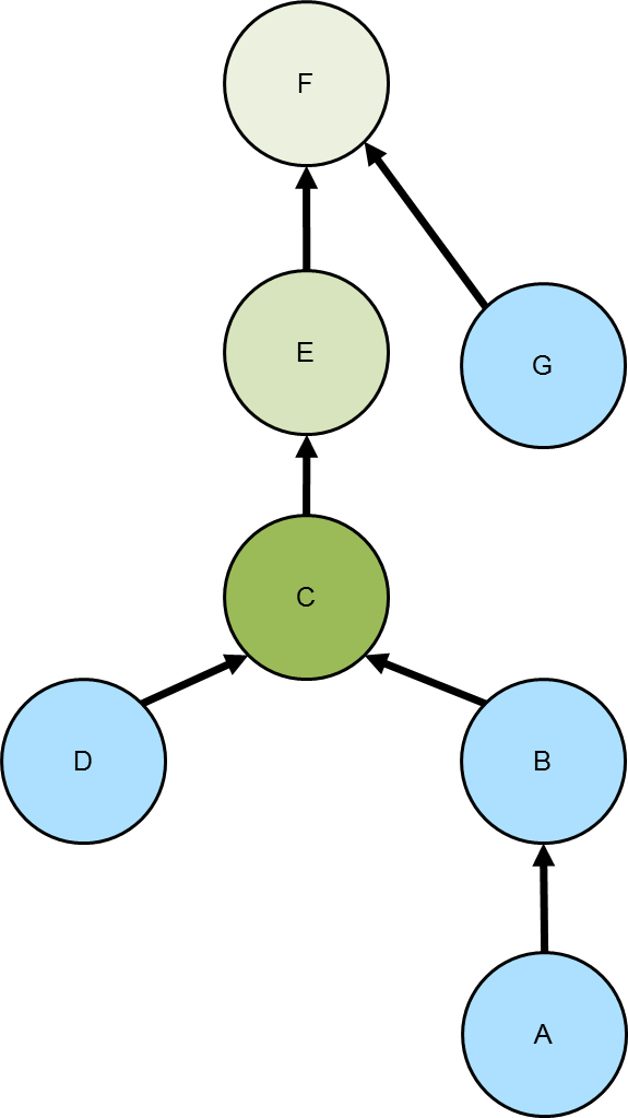 Given a tree, the lowest common ancestor
is the deepest vertex that is common to two or more other vertices. The diagram to the right depicts the common
ancestor tree for vertices A and D in the various green shades. The C vertex, the vertex with the darkest green
shading, is the lowest common ancestor.
Given a tree, the lowest common ancestor
is the deepest vertex that is common to two or more other vertices. The diagram to the right depicts the common
ancestor tree for vertices A and D in the various green shades. The C vertex, the vertex with the darkest green
shading, is the lowest common ancestor.
The following code simply sets up the graph depicted above using "hasParent" for the edge label:
gremlin> g.addV().property(id, 'A').as('a').
           addV().property(id, 'B').as('b').
           addV().property(id, 'C').as('c').
           addV().property(id, 'D').as('d').
           addV().property(id, 'E').as('e').
           addV().property(id, 'F').as('f').
           addV().property(id, 'G').as('g').
           addE('hasParent').from('a').to('b').
           addE('hasParent').from('b').to('c').
           addE('hasParent').from('d').to('c').
           addE('hasParent').from('c').to('e').
           addE('hasParent').from('e').to('f').
           addE('hasParent').from('g').to('f').iterate()
Given that graph, the following traversal will get the lowest common ancestor for two vertices, A and D:
gremlin> g.V('A').
           repeat(out('hasParent')).emit().as('x').
           repeat(__.in('hasParent')).emit(hasId('D')).
           select('x').limit(1)
==>v[C]
The above traversal is reasonably straightforward to follow in that it simply traverses up the tree from the A vertex and then traverses down from each ancestor until it finds the "D" vertex. The first path that uncovers that match is the lowest common ancestor.
The complexity of finding the lowest common ancestor increases when trying to find the ancestors of three or more vertices.
gremlin> input = ['A','B','D']
==>A
==>B
==>D
gremlin> g.V(input.head()).
           repeat(out('hasParent')).emit().as('x'). //1\
           V().has(id, within(input.tail())). //2\
           repeat(out('hasParent')).emit(where(eq('x'))). //3\
           group().
             by(select('x')).
             by(path().count(local).fold()). //4\
           unfold().filter(select(values).count(local).is(input.tail().size())). //5\
           order().by(select(values).
           unfold().sum()). //6\
           select(keys).limit(1) //7\
==>v[C]-
The start of the traversal is not so different than the previous one and starts with vertex A.
-
Use a mid-traversal
V()to find the child vertices B and D. -
Traverse up the tree for B and D and find common ancestors that were labeled with "x".
-
Group on the common ancestors where the value of the grouping is the length of the path.
-
The result of the previous step is a
Mapwith a vertex (i.e. common ancestor) for the key and a list of path lengths. Unroll theMapand ensure that the number of path lengths are equivalent to the number of children that were given to the mid-traversalV(). -
Order the results based on the sum of the path lengths.
-
Since the results were placed in ascending order, the first result must be the lowest common ancestor.
As the above traversal utilizes a mid-traversal V(), it cannot be used for OLAP. In OLAP, the pattern changes a bit:
gremlin> g.withComputer().
           V().has(id, within(input)).
           aggregate('input').hasId(input.head()). //1\
           repeat(out('hasParent')).emit().as('x').
           select('input').unfold().has(id, within(input.tail())).
           repeat(out('hasParent')).emit(where(eq('x'))).
           group().
             by(select('x')).
             by(path().count(local).fold()).
           unfold().filter(select(values).count(local).is(input.tail().size())).
           order().
             by(select(values).unfold().sum()).
           select(keys).limit(1)
==>v[C]-
The main difference for OLAP is the use of
aggregate()over the mid-traversalV().
Maximum Depth
Finding the maximum depth of a tree starting from a specified root vertex can be determined as follows:
gremlin> g.addV().property('name', 'A').as('a').
           addV().property('name', 'B').as('b').
           addV().property('name', 'C').as('c').
           addV().property('name', 'D').as('d').
           addV().property('name', 'E').as('e').
           addV().property('name', 'F').as('f').
           addV().property('name', 'G').as('g').
           addE('hasParent').from('a').to('b').
           addE('hasParent').from('b').to('c').
           addE('hasParent').from('d').to('c').
           addE('hasParent').from('c').to('e').
           addE('hasParent').from('e').to('f').
           addE('hasParent').from('g').to('f').iterate()
gremlin> g.V().has('name','F').repeat(__.in()).emit().path().count(local).max()
==>5
gremlin> g.V().has('name','C').repeat(__.in()).emit().path().count(local).max()
==>3
The traversals shown above are fairly straightforward. The traversal
beings at a particular starting vertex, traverse in on the "hasParent" edges emitting all vertices as it goes. It
calculates the path length and then selects the longest one. While this approach is quite direct, there is room for
improvement:
gremlin> g.V().has('name','F').
           repeat(__.in()).emit(__.not(inE())).tail(1).
           path().count(local)
==>5
gremlin> g.V().has('name','C').
           repeat(__.in()).emit(__.not(inE())).tail(1).
           path().count(local)
==>3
There are two optimizations at play. First, there is no need to emit all the vertices, only the "leaf" vertices (i.e. those without incoming edges). Second, all results save the last one can be ignored to that point (i.e. the last one is the one at the deepest point in the tree). In this way, the path and path length only need to be calculated for a single result.
The previous approaches to calculating the maximum depth use path calculations to achieve the answer. Path calculations
can be expensive and if possible avoided if they are not needed. Another way to express a traversal that calculates
the maximum depth is to use the sack() step:
gremlin> g.withSack(1).V().has('name','F').
           repeat(__.in().sack(sum).by(constant(1))).emit().
           sack().max()
==>5
gremlin> g.withSack(1).V().has('name','C').
           repeat(__.in().sack(sum).by(constant(1))).emit().
           sack().max()
==>3
Time-based Indexing
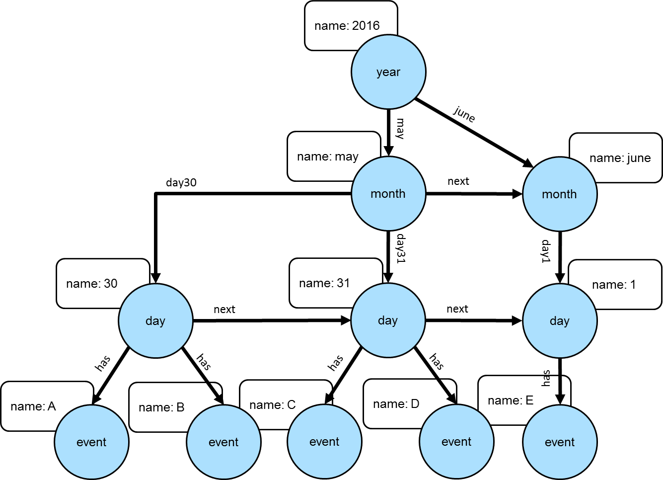
Trees can be used for modeling time-oriented data in a graph. Modeling time where there are "year", "month" and "day" vertices (or lower granularity as needed) allows the structure of the graph to inherently index data tied to them.
|
Note
|
This model is discussed further in this Neo4j blog post. Also, there can be other versions of this model that utilize different edge/vertex labeling and property naming strategies. The schema depicted here is designed for simplicity. |
The Gremlin script below creates the graph depicted in the graph above:
gremlin> g.addV('year').property('name', '2016').as('y2016').
           addV('month').property('name', 'may').as('m05').
           addV('month').property('name', 'june').as('m06').
           addV('day').property('name', '30').as('d30').
           addV('day').property('name', '31').as('d31').
           addV('day').property('name', '01').as('d01').
           addV('event').property('name', 'A').as('eA').
           addV('event').property('name', 'B').as('eB').
           addV('event').property('name', 'C').as('eC').
           addV('event').property('name', 'D').as('eD').
           addV('event').property('name', 'E').as('eE').
           addE('may').from('y2016').to('m05').
           addE('june').from('y2016').to('m06').
           addE('day30').from('m05').to('d30').
           addE('day31').from('m05').to('d31').
           addE('day01').from('m06').to('d01').
           addE('has').from('d30').to('eA').
           addE('has').from('d30').to('eB').
           addE('has').from('d31').to('eC').
           addE('has').from('d31').to('eD').
           addE('has').from('d01').to('eE').
           addE('next').from('d30').to('d31').
           addE('next').from('d31').to('d01').
addE('next').from('m05').to('m06').iterate()|
Important
|
The code example above does not create any indices. Proper index creation, which is specific to the graph implementation used, will be critical to the performance of traversals over this structure. |
gremlin> g.V().has('name','2016').out().out().out('has').values() //1\
==>E
==>C
==>D
==>A
==>B
gremlin> g.V().has('name','2016').out('may').out().out('has').values() //2\
==>C
==>D
==>A
==>B
gremlin> g.V().has('name','2016').out('may').out('day31').out('has').values() //3\
==>C
==>D
gremlin> g.V().has('name','2016').out('may').out('day31').as('start').
           V().has('name','2016').out('june').out('day01').as('end').
           emit().repeat(__.in('next')).until(where(eq('start'))).
           out('has').
           order().by('name').values('name') //4\
==>C
==>D
==>E-
Find all the events in 2016.
-
Find all the events in May of 2016.
-
Find all the events on May 31, 2016.
-
Find all the events between May 31, 2016 and June 1, 2016.
OLAP traversals with Spark on YARN
TinkerPop’s combination of SparkGraphComputer
and HadoopGraph allows for running
distributed, analytical graph queries (OLAP) on a computer cluster. The
reference documentation covers the cases
where Spark runs locally or where the cluster is managed by a Spark server. However, many users can only run OLAP jobs
via the Hadoop 2.x Resource Manager (YARN), which requires SparkGraphComputer to be
configured differently. This recipe describes this configuration.
Approach
Most configuration problems of TinkerPop with Spark on YARN stem from three reasons:
-
SparkGraphComputercreates its ownSparkContextso it does not get any configs from the usualspark-submitcommand. -
The TinkerPop Spark plugin did not include Spark on YARN runtime dependencies until version 3.2.7/3.3.1.
-
Resolving reason 2 by adding the cluster’s
spark-assemblyjar to the classpath creates a host of version conflicts, because Spark 1.x dependency versions have remained frozen since 2014.
The current recipe follows a minimalist approach in which no dependencies are added to the dependencies included in the TinkerPop binary distribution. The Hadoop cluster’s Spark installation is completely ignored. This approach minimizes the chance of dependency version conflicts.
Prerequisites
This recipe is suitable for both a real external and a local pseudo Hadoop cluster. While the recipe is maintained for the vanilla Hadoop pseudo-cluster, it has been reported to work on real clusters with Hadoop distributions from various vendors.
If you want to try the recipe on a local Hadoop pseudo-cluster, the easiest way to install
it is to look at the install script at https://github.com/apache/tinkerpop/blob/3.2.7-SNAPSHOT/docker/hadoop/install.sh
and the start hadoop section of https://github.com/apache/tinkerpop/blob/3.2.7-SNAPSHOT/docker/scripts/build.sh.
This recipe assumes that you installed the Gremlin Console with the
Spark plugin (the
Hadoop plugin is optional). Your Hadoop cluster
may have been configured to use file compression, e.g. LZO compression. If so, you need to copy the relevant
jar (e.g. hadoop-lzo-*.jar) to Gremlin Console’s ext/spark-gremlin/lib folder.
For starting the Gremlin Console in the right environment, create a shell script (e.g. bin/spark-yarn.sh) with the
contents below. Of course, actual values for GREMLIN_HOME, HADOOP_HOME and HADOOP_CONF_DIR need to be adapted to
your particular environment.
#!/bin/bash
# Variables to be adapted to the actual environment
GREMLIN_HOME=/home/yourdir/lib/apache-tinkerpop-gremlin-console-3.2.7-SNAPSHOT-standalone
export HADOOP_HOME=/usr/local/lib/hadoop-2.7.2
export HADOOP_CONF_DIR=/usr/local/lib/hadoop-2.7.2/etc/hadoop

# Have TinkerPop find the hadoop cluster configs and hadoop native libraries
export CLASSPATH=$HADOOP_CONF_DIR
export JAVA_OPTIONS="-Djava.library.path=$HADOOP_HOME/lib/native:$HADOOP_HOME/lib/native/Linux-amd64-64"

# Start gremlin-console without getting the HADOOP_GREMLIN_LIBS warning
cd $GREMLIN_HOME
[ ! -e empty ] && mkdir empty
export HADOOP_GREMLIN_LIBS=$GREMLIN_HOME/empty
bin/gremlin.sh
Running the job
You can now run a gremlin OLAP query with Spark on YARN:
$ hdfs dfs -put data/tinkerpop-modern.kryo .
$ . bin/spark-yarn.sh
gremlin> hadoop = System.getenv('HADOOP_HOME')
gremlin> hadoopConfDir = System.getenv('HADOOP_CONF_DIR')
gremlin> archive = 'spark-gremlin.zip'
==>spark-gremlin.zip
gremlin> archivePath = "/tmp/$archive"
==>/tmp/spark-gremlin.zip
gremlin> ['bash', '-c', "rm $archivePath 2>/dev/null; cd ext/spark-gremlin/lib && zip $archivePath *.jar"].execute()
==>java.lang.UNIXProcess@633fd91
gremlin> conf = new PropertiesConfiguration('conf/hadoop/hadoop-gryo.properties')
==>org.apache.commons.configuration.PropertiesConfiguration@697173d9
gremlin> conf.setProperty('spark.master', 'yarn-client')
gremlin> conf.setProperty('spark.yarn.dist.archives', "$archivePath")
gremlin> conf.setProperty('spark.yarn.appMasterEnv.CLASSPATH', "./$archive/*:$hadoopConfDir")
gremlin> conf.setProperty('spark.executor.extraClassPath', "./$archive/*:$hadoopConfDir")
gremlin> conf.setProperty('spark.driver.extraLibraryPath', "$hadoop/lib/native:$hadoop/lib/native/Linux-amd64-64")
gremlin> conf.setProperty('spark.executor.extraLibraryPath', "$hadoop/lib/native:$hadoop/lib/native/Linux-amd64-64")
gremlin> conf.setProperty('gremlin.spark.persistContext', 'true')
gremlin> graph = GraphFactory.open(conf)
==>hadoopgraph[gryoinputformat->gryooutputformat]
gremlin> g = graph.traversal().withComputer(SparkGraphComputer)
==>graphtraversalsource[hadoopgraph[gryoinputformat->gryooutputformat], sparkgraphcomputer]
gremlin> g.V().group().by(values('name')).by(both().count())
==>[ripple:1,peter:1,vadas:1,josh:3,lop:3,marko:3]If you run into exceptions, you will have to dig into the logs. You can do this from the command line with
yarn application -list -appStates ALL to find the applicationId, while the logs are available with
yarn logs -applicationId application_1498627870374_0008. Alternatively, you can inspect the logs via
the YARN Resource Manager UI (e.g. http://rm.your.domain:8088/cluster), provided that YARN was configured with the
yarn.log-aggregation-enable property set to true. See the Spark documentation for
additional hints.
Explanation
This recipe does not require running the bin/hadoop/init-tp-spark.sh script described in the
reference documentation and thus is also
valid for cluster users without access permissions to do so.
Rather, it exploits the spark.yarn.dist.archives property, which points to an archive with jars on the local file
system and is loaded into the various YARN containers. As a result the spark-gremlin.zip archive becomes available
as the directory named spark-gremlin.zip in the YARN containers. The spark.executor.extraClassPath and
spark.yarn.appMasterEnv.CLASSPATH properties point to the files inside this archive.
This is why they contain the ./spark-gremlin.zip/* item. Just because a Spark executor got the archive with
jars loaded into its container, does not mean it knows how to access them.
Also the HADOOP_GREMLIN_LIBS mechanism is not used because it can not work for Spark on YARN as implemented (jars
added to the SparkContext are not available to the YARN application master).
The gremlin.spark.persistContext property is explained in the reference documentation of
SparkGraphComputer: it helps in getting
follow-up OLAP queries answered faster, because you skip the overhead for getting resources from YARN.
Additional configuration options
This recipe does most of the graph configuration in the Gremlin Console so that environment variables can be used and
the chance of configuration mistakes is minimal. Once you have your setup working, it is probably easier to make a copy
of the conf/hadoop/hadoop-gryo.properties file and put the property values specific to your environment there. This is
also the right moment to take a look at the spark-defaults.xml file of your cluster, in particular the settings for
the Spark History Service, which allows you to access logs of
finished applications via the YARN resource manager UI.
This recipe uses the Gremlin Console, but things should not be very different for your own JVM-based application,
as long as you do not use the spark-submit or spark-shell commands. You will also want to check the additional
runtime dependencies listed in the Gremlin-Plugin-Dependencies section of the manifest file in the spark-gremlin
jar.
You may not like the idea that the Hadoop and Spark jars from the TinkerPop distribution differ from the versions in
your cluster. If so, just build TinkerPop from source with the corresponding dependencies changed in the various pom.xml
files (e.g. spark-core_2.10-1.6.1-some-vendor.jar instead of spark-core_2.10-1.6.1.jar). Of course, TinkerPop will
only build for exactly matching or slightly differing artifact versions.
Implementation Recipes
Style Guide
Gremlin is a data flow language where each new step concatenation alters the stream accordingly. This aspect of the language allows users to easily "build-up" a traversal (literally) step-by-step until the expected results are returned. For instance:
gremlin> g.V(1)
==>v[1]
gremlin> g.V(1).out('knows')
==>v[2]
==>v[4]
gremlin> g.V(1).out('knows').out('created')
==>v[5]
==>v[3]
gremlin> g.V(1).out('knows').out('created').groupCount()
==>[v[3]:1,v[5]:1]
gremlin> g.V(1).out('knows').out('created').groupCount().by('name')
==>[ripple:1,lop:1]
A drawback of building up a traversal is that users tend to create long, single line traversal that are hard to read. For simple traversals, a single line is fine. For complex traversals, there are few formatting patterns that should be followed which will yield cleaner, easier to understand traversals. For instance, the last traversal above would be written:
gremlin> g.V(1).out('knows').out('created').
           groupCount().by('name')
==>[ripple:1,lop:1]
Lets look at a complex traversal and analyze each line according to the recommended formatting rule is subscribes to.
gremlin> g.V().out('knows').out('created'). //1\
           group().by('lang').by(). //2\
             select('java').unfold(). //3\
           in('created').hasLabel('person'). //4\
           order(). //5\
             by(inE().count(),decr). //6\
             by('age',incr).
           dedup().limit(10).values('name') //7\
==>josh
==>marko
==>peter-
A sequence of
ins().outs().filters().etc()on a single line until it gets too long. -
When a barrier (reducer, aggregator, etc.) is used, put it on a new line.
-
When a next line component is an "add on" to the previous line component, 2 space indent. The
select()-step in this context is "almost like" aby()-modulator as its projecting data out of thegroup(). Theunfold()-step is a data formatting necessity that should not be made too prominent. -
Back to a series of
ins().outs().filters().etc()on a single line. -
order()is a barrier step and thus, should be on a new line. -
If there is only one
by()-modulator (or a series of short ones), keep it on one line, else eachby()is a new line. -
Back to a series
ins().outs().filters().etc().
Style Guide Rules
A generalization of the specifics above are presented below.
-
Always use 2 space indent.
-
No newline should ever have the same indent as the line starting with the traversal source
g. -
Barrier steps should form line breaks unless they are simple (e.g.
sum()). -
Complex
by()-modulators form indented "paragraphs." -
Standard filters, maps, flatMaps remain on the same line until they get too long.
Given the diversity of traversals and the complexities introduced by lambdas (for example), these rules will not always lead to optimal representations. However, by in large, the style rules above will help make 90% of traversals look great.
Traversal Component Reuse
Good software development practices require reuse to keep software maintainable. In Gremlin, there are often bits of
traversal logic that could be represented as components that might be tested independently and utilized
as part of other traversals. One approach to doing this would be to extract such logic into an anonymous traversal
and provide it to a parent traversal through flatMap() step.
Using the modern toy graph as an example, assume that there are number of traversals that are interested in filtering on edges where the "weight" property is greater than "0.5". A query like that might look like this:
gremlin> g.V(1).outE("knows").has('weight', P.gt(0.5d)).inV().both()
==>v[5]
==>v[3]
==>v[1]
Repeatedly requiring that filter on "weight" could lead to a lot of duplicate code, which becomes difficult to maintain. It would be nice to extract that logic so as to centralize it for reuse in all places where needed. An anonymous traversal allows that to happen and can be created as follows.
gremlin> weightFilter = outE("knows").has('weight', P.gt(0.5d)).inV();[]
gremlin> g.V(1).flatMap(weightFilter).both()
==>v[5]
==>v[3]
==>v[1]
The weightFilter is an anonymous traversal and it is created by way class. The is omitted above from
initalization of weightFilter because it is statically imported to the Gremlin Console. The weightFilter gets
passed to the "full" traversal by way for flatMap() step and the results are the same. Of course, there is a problem.
If there is an attempt to use that weightFilter a second time, the traversal with thrown an exception because both
the weightFilter and parent traversal have been "compiled" which prevents their re-use. A simple fix to this would
be to clone the weightFilter.
gremlin> weightFilter = outE("knows").has('weight', P.gt(0.5d)).inV();[]
gremlin> g.V(1).flatMap(weightFilter.clone()).both()
==>v[5]
==>v[3]
==>v[1]
gremlin> g.V(1).flatMap(weightFilter.clone()).bothE().otherV()
==>v[5]
==>v[3]
==>v[1]
gremlin> g.V(1).flatMap(weightFilter.clone()).groupCount()
==>[v[4]:1]
Now the weightFilter can be reused over and over again. Remembering to clone() might lead to yet another maintenance
issue in that failing to recall that step would likely result in a bug. One option might be to wrap the weightFilter
creation in a function that returns the clone. Another approach might be to parameterize that function to construct
a new anonymous traversal each time with the idea being that this might gain even more flexibility in parameterizing
the anonymous traversal itself.
gremlin> weightFilter = { w -> outE("knows").has('weight', P.gt(w)).inV() }
==>groovysh_evaluate$_run_closure1@286090c
gremlin> g.V(1).flatMap(weightFilter(0.5d)).both()
==>v[5]
==>v[3]
==>v[1]
gremlin> g.V(1).flatMap(weightFilter(0.5d)).bothE().otherV()
==>v[5]
==>v[3]
==>v[1]
gremlin> g.V(1).flatMap(weightFilter(0.5d)).groupCount()
==>[v[4]:1]
How to Contribute a Recipe
Recipes are generated under the same system as all TinkerPop documentation and is stored directly in the source code repository. TinkerPop documentation is all asciidoc based and can be generated locally with either shell script/Maven or Docker build commands. Once changes are complete, submit a pull request for review by TinkerPop committers.
|
Note
|
Please review existing recipes and attempt to conform to their writing and visual style. It may also be a good idea to discuss ideas for a recipe on the developer mailing list prior to starting work on it, as the community might provide insight on the approach and idea that would be helpful. It is preferable that a JIRA issue be opened that describes the nature of the recipe so that the eventual pull request can be bound to that issue. |
|
Important
|
Please read TinkerPop’s policy on contributing prior to submitting a recipe. |
To contribute a recipe, first clone the repository:
git clone https://github.com/apache/tinkerpop.gitThe recipes can be found in this directory:
ls docs/src/recipesEach recipe exists within a separate .asciidoc file. The file name should match the name of the recipe. Recipe names
should be short, but descriptive (as they need to fit in the left-hand table of contents when generated). The
index.asciidoc is the parent document that "includes" the content of each individual recipe file. A recipe file is
included in the index.asciidoc with an entry like this: include::my-recipe.asciidoc[]
Documentation should be generated locally for review prior to submitting a pull request. TinkerPop documentation is
"live" in that it is bound to a specific version when generated. Furthermore, code examples (those that are
gremlin-groovy based) are executed at document generation time with the results written directly into the output.
The following command will generate the documentation with:
bin/process-docs.shThe generated documentation can be found at target/docs/htmlsingle/recipes. This process can be long on the first
run of the documentation as it is generating all of the documentation locally (e.g. reference documentation,
tutorials, etc). To generate just the recipes, follow this process:
bin/process-docs.sh -f docs/src/recipesThe bin/process-docs.sh approach requires that Hadoop is installed. To avoid that prerequisite, try using Docker:
docker/build.sh -dThe downside to using Docker is that the process will take longer as each run will require the entire documentation set to be generated.
The final step to submitting a recipe is to issue a pull request through GitHub. It is helpful to prefix the name of the pull request with the JIRA issue number, so that TinkerPop’s automation between GitHub and JIRA are linked. As mentioned earlier in this section, the recipe will go under review by TinkerPop committers prior to merging. This process may take several days to complete. We look forward to receiving your submissions!
Appendix
Many of the recipes are based on questions and answers provided on the gremlin-users mailing list or on StackOverflow. This section contains those traversals from those sources that do not easily fit any particular pattern (i.e. a recipe), but are nonetheless interesting and thus remain good tools for learning Gremlin.
For each person in a "follows" graph, determine the number of followers and list their names.
gremlin> g.addV().property('name','marko').as('marko').
           addV().property('name','josh').as('josh').
           addV().property('name','daniel').as('daniel').
           addV().property('name','matthias').as('matthias').
           addE('follows').from('josh').to('marko').
           addE('follows').from('matthias').to('josh').
           addE('follows').from('daniel').to('josh').
           addE('follows').from('daniel').to('marko').iterate()
gremlin> g.V().as('p').
           map(__.in('follows').values('name').fold()).
           project('person','followers','numFollowers').
             by(select('p').by('name')).
             by().
             by(count(local))
==>[person:marko,followers:[josh,daniel],numFollowers:2]
==>[person:josh,followers:[matthias,daniel],numFollowers:2]
==>[person:daniel,followers:[],numFollowers:0]
==>[person:matthias,followers:[],numFollowers:0]
It might also be alternatively written as:
gremlin> g.V().group().
                 by('name').
                 by(project('numFollowers','followers').
                      by(__.in('follows').count()).
                      by(__.in('follows').values('name').fold())).next()
==>daniel={numFollowers=0, followers=[]}
==>matthias={numFollowers=0, followers=[]}
==>josh={numFollowers=2, followers=[matthias, daniel]}
==>marko={numFollowers=2, followers=[josh, daniel]}
or even:
gremlin> g.V().group().
                 by('name').
                 by(__.in('follows').values('name').fold().
                     project('numFollowers','followers').
                       by(count(local)).
                       by()).next()
==>daniel={numFollowers=0, followers=[]}
==>matthias={numFollowers=0, followers=[]}
==>josh={numFollowers=2, followers=[matthias, daniel]}
==>marko={numFollowers=2, followers=[josh, daniel]}
In the "modern" graph, show each person, the software they worked on and the co-worker count for the software and the names of those co-workers.
gremlin> g.V().hasLabel("person").as("p").
           out("created").as("s").
           map(__.in("created").
             where(neq("p")).values("name").fold()).
           group().by(select("p").by("name")).
             by(group().by(select("s").by("name")).
             by(project("numCoworkers","coworkers").
                  by(count(local)).by())).next()
==>peter={lop={numCoworkers=2, coworkers=[marko, josh]}}
==>josh={ripple={numCoworkers=0, coworkers=[]}, lop={numCoworkers=2, coworkers=[marko, peter]}}
==>marko={lop={numCoworkers=2, coworkers=[josh, peter]}}
Assuming a graph of students, classes and times, detect students who have a conflicting schedule.
gremlin> g.addV("student").property("name", "Pete").as("s1").
           addV("student").property("name", "Joe").as("s2").
           addV("class").property("name", "Java's GC").as("c1").
           addV("class").property("name", "FP Principles").as("c2").
           addV("class").property("name", "Memory Management in C").as("c3").
           addV("class").property("name", "Memory Management in C++").as("c4").
           addV("timeslot").property("date", "11/25/2016").property("fromTime", "10:00").property("toTime", "11:00").as("t1").
           addV("timeslot").property("date", "11/25/2016").property("fromTime", "11:00").property("toTime", "12:00").as("t2").
           addE("attends").from("s1").to("c1").
           addE("attends").from("s1").to("c2").
           addE("attends").from("s1").to("c3").
           addE("attends").from("s1").to("c4").
           addE("attends").from("s2").to("c2").
           addE("attends").from("s2").to("c3").
           addE("allocated").from("c1").to("t1").
           addE("allocated").from("c1").to("t2").
           addE("allocated").from("c2").to("t1").
           addE("allocated").from("c3").to("t2").
           addE("allocated").from("c4").to("t2").iterate()
gremlin> g.V().hasLabel("student").as("s").
           out("attends").as("c").
           out("allocated").as("t").
           select("s").
           out("attends").
           where(neq("c")).
           out("allocated").
           where(eq("t")).
           group().
             by(select("s").by("name")).
             by(group().by(select("t").by(valueMap("fromTime","toTime"))).
                        by(select("c").dedup().values("name").fold())).next()
==>Pete={{fromTime=[10:00], toTime=[11:00]}=[Java's GC, FP Principles], {fromTime=[11:00], toTime=[12:00]}=[Memory Management in C, Memory Management in C++, Java's GC]}
In the "modern" graph, with a duplicate edge added, find the vertex pairs that have more than one edge between them.
gremlin> g.V(1).as("a").V(3).addE("created").property("weight",0.4d).from("a").iterate()
gremlin> g.V(1).outE("created")
==>e[9][1-created->3]
==>e[13][1-created->3]
gremlin> g.V().as("a").
           out().as("b").
           groupCount().
             by(select("a","b")).
           unfold().
           filter(select(values).is(gt(1))).
           select(keys)
==>[a:v[1],b:v[3]]
The following example assumes that the edges point in the OUT direction. Assuming undirected edges:
gremlin> g.V().where(without("x")).as("a").
           outE().as("e").inV().as("b").
           filter(bothE().where(neq("e")).otherV().where(eq("a"))).store("x").
           select("a","b").dedup()
In the "crew" graph, find vertices that match on a complete set of multi-properties.
gremlin> places = ["centreville","dulles"];[]  // will not match as "purcellville" is missing
gremlin> g.V().not(has("location", without(places))).
           where(values("location").is(within(places)).count().is(places.size())).
           valueMap()
gremlin> places = ["centreville","dulles","purcellville"];[]
gremlin> g.V().not(has("location", without(places))).
           where(values("location").is(within(places)).count().is(places.size())).
           valueMap()
==>[name:[stephen],location:[centreville,dulles,purcellville]]
Methods for performing some basic mathematical operations in the "modern" graph.
gremlin> g.V().values("age").sum() // sum all ages
==>123
gremlin> g.V().values("age").fold(1, mult) // multiply all ages
==>876960
gremlin> g.withSack(0).V().values("age").sack(sum).sack(sum).by(constant(-1)).sack() // subtract 1
==>28
==>26
==>31
==>34
gremlin> g.withSack(0).V().values("age").sack(sum).sack(sum).sack() // multiply by 2 (simple)
==>58
==>54
==>64
==>70
gremlin> g.withSack(0).V().values("age").sack(sum).sack(mult).by(constant(2)).sack() // multiply by 2 (generally useful for multiplications by n)
==>58
==>54
==>64
==>70
Method for doing a sum with division.
gremlin> g.addV().property(id, "a").as("a").
           addV().property(id, "b").as("b").
           addE("link").from("a").to("b").
           addE("link").from("b").to("a").
           addE("link").from("b").to("a").iterate()
gremlin> g.withSack(0d).
            V("a").as("a").
            V("b").as("b").
              project("ab", "ba").
                by(inE("link").where(outV().as("a")).count()).
                by(outE("link").where(inV().as("a")).count()).
              sack(sum).by(select("ab")).
              sack(div).by(select("ba")).
              project("a", "b", "#(a,b)", "#(b,a)", "#(a,b) / #(b,a)").
                by(select("a")).
                by(select("b")).
                by(select("ab")).
                by(select("ba")).
                by(sack())
==>[a:v[a],b:v[b],#(a,b):1,#(b,a):2,#(a,b) / #(b,a):0.5]
Dropping a vertex, as well as the vertices related to that dropped vertex that are connected by a "knows" edge in the "modern" graph
gremlin> g.V().has('name','marko').outE()
==>e[9][1-created->3]
==>e[7][1-knows->2]
==>e[8][1-knows->4]
gremlin> g.V().has('name','marko').sideEffect(out('knows').drop()).drop()
gremlin> g.V().has('name','marko')
gremlin> g.V(2,4,3)
==>v[3]
For the specified graph, find all neighbor vertices connected to "A" as filtered by datetime, those neighbor vertices that don’t have datetime vertices, and those neighbor vertices that have the label "dimon".
gremlin> g.addV().property("name", "A").as("a").
           addV().property("name", "B").as("b").
           addV().property("name", "C").as("c").
           addV().property("name", "D").as("d").
           addV().property("name", "E").as("e").
           addV("dimon").property("name", "F").as("f").
           addV().property("name", "G").as("g").property("date", 20160818).
           addV().property("name", "H").as("h").property("date", 20160817).
           addE("rel").from("a").to("b").
           addE("rel").from("a").to("c").
           addE("rel").from("a").to("d").
           addE("rel").from("a").to("e").
           addE("rel").from("c").to("f").
           addE("occured_at").from("d").to("g").
           addE("occured_at").from("e").to("h").iterate()
gremlin> // D and E have a valid datetime
==>true
gremlin> g.V().has("name", "A").out("rel").
           union(where(out("occured_at").has("date", gte(20160817))),
                 __.not(outE("occured_at")).coalesce(out().hasLabel("dimon"), identity())).
           valueMap()
==>[name:[B]]
==>[name:[F]]
==>[name:[D]]
==>[name:[E]]
gremlin> // only E has a valid date
==>true
gremlin> g.V().has("name", "A").out("rel").
           union(where(out("occured_at").has("date", lte(20160817))),
                 __.not(outE("occured_at")).coalesce(out().hasLabel("dimon"), identity())).
           valueMap()
==>[name:[B]]
==>[name:[F]]
==>[name:[E]]
gremlin> // only D has a valid date
==>true
gremlin> g.V().has("name", "A").out("rel").
           union(where(out("occured_at").has("date", gt(20160817))),
                 __.not(outE("occured_at")).coalesce(out().hasLabel("dimon"), identity())).
           valueMap()
==>[name:[B]]
==>[name:[F]]
==>[name:[D]]
gremlin> // neither D nor E have a valid date
==>true
gremlin> g.V().has("name", "A").out("rel").
           union(where(out("occured_at").has("date", lt(20160817))),
                 __.not(outE("occured_at")).coalesce(out().hasLabel("dimon"), identity())).
           valueMap()
==>[name:[B]]
==>[name:[F]]
Use element labels in a select.
gremlin> g.V(1).as("a").
           both().
           map(group().by(label).by(unfold())).as("b").
           select("a","b").
           map(union(project("a").by(select("a")), select("b")).
           unfold().
           group().
             by(select(keys)).
             by(select(values)))
==>[a:v[1],software:v[3]]
==>[a:v[1],person:v[2]]
==>[a:v[1],person:v[4]]
gremlin> g.V().as("a").
           both().
           map(group().by(label).by(unfold())).as("b").
           select("a","b").
           group().
             by(select("a")).
             by(select("b").
                  group().
                    by(select(keys)).
                    by(select(values).fold())).
             unfold().
             map(union(select(keys).project("a").by(), select(values)).
             unfold().
             group().
               by(select(keys).unfold()).
               by(select(values).unfold().unfold().fold()))
==>[a:[v[1]],software:[v[3]],person:[v[2],v[4]]]
==>[a:[v[2]],person:[v[1]]]
==>[a:[v[3]],person:[v[1],v[4],v[6]]]
==>[a:[v[4]],software:[v[5],v[3]],person:[v[1]]]
==>[a:[v[5]],person:[v[4]]]
==>[a:[v[6]],software:[v[3]]]
Sum edge weight with a coefficient.
gremlin> g.addV('person').property('name','alice').as('alice').
           addV('person').property('name','bobby').as('bobby').
           addV('person').property('name','cindy').as('cindy').
           addV('person').property('name','david').as('david').
           addV('person').property('name','eliza').as('eliza').
           addE('rates').from('alice').to('bobby').property('tag','ruby').property('value',9).
           addE('rates').from('bobby').to('cindy').property('tag','ruby').property('value',8).
           addE('rates').from('cindy').to('david').property('tag','ruby').property('value',7).
           addE('rates').from('david').to('eliza').property('tag','ruby').property('value',6).
           addE('rates').from('alice').to('eliza').property('tag','java').property('value',9).iterate()
gremlin>  g.withSack(1.0).V().has("name","alice").
            repeat(outE("rates").has("tag","ruby").
                   project("a","b","c").
                     by(inV()).
                     by(sack()).
                     by("value").as("x").
                   select("a").
                   sack(mult).by(constant(0.5))).
               times(3).emit().
             select(all, "x").
             project("name","score").
               by(tail(local, 1).select("a").values("name")).
               by(unfold().
                  sack(assign).by(select("b")).
                  sack(mult).by(select("c")).
                  sack().sum())
==>[name:bobby,score:9.0]
==>[name:cindy,score:13.00]
==>[name:david,score:14.750]